
State Occupancy Probabilities with Proportional-Odds Models
Source:vignettes/full-po-sops.Rmd
full-po-sops.RmdMany clinical trials record a patient’s condition repeatedly on an ordered scale, for example once a day from “at home” to “dead”. A natural way to summarize such data is the state occupancy probability (SOP): the probability that a patient is in a given state on a given day. Comparing SOPs between treatment arms shows when, and in which states, a treatment makes a difference.
mostr estimates SOPs from a transition model: an ordinal regression that predicts tomorrow’s state from today’s state, treatment, time, and other covariates. Chaining these one-day predictions together gives the probability of each state on every later day. This article walks through the complete workflow:
- simulate and prepare longitudinal data;
- fit a proportional-odds transition model;
- estimate SOPs for each treatment arm, with confidence intervals;
- check whether the fitted model reproduces features of the observed data.
We fit the same model twice, once with vglm_markov()
(using the VGAM package) and once with orm_markov() (using
the rms package), to show that both give the same answer.
Example data
We simulate daily health states for 400 patients over 28 days. The
simulation model is based on data from the Adaptive COVID-19 Treatment
Trial 2 (ACTT-2), which enrolled adults hospitalized with moderate
to severe COVID-19,1 so the simulated trajectories resemble
those seen in the trial. We choose the treatment effect ourselves:
treatment_effect = log(0.8) means that, on any day, treated
patients have 0.8 times the odds of being in a worse state than control
patients who started the day in the same state.
States follow the trial’s NIAID eight-point ordinal scale. Higher numbers indicate worse health:
| State | Meaning |
|---|---|
| 1 | Outside hospital, with usual activities unrestricted |
| 2 | Outside hospital, with restricted activities, oxygen at home, or both |
| 3 | In hospital, without oxygen and no further medical care needed |
| 4 | In hospital, without oxygen but still needing medical care |
| 5 | In hospital, needing supplemental oxygen |
| 6 | In hospital, needing high-flow oxygen or noninvasive ventilation |
| 7 | In hospital, needing invasive ventilation or extracorporeal membrane oxygenation (ECMO) |
| 8 | Death |
Death is an absorbing state: once a patient enters it, they stay there for the rest of follow-up.
The simulated data have one row per patient and day, with the columns
that mostr expects by default: id (patient),
time (day), y (state on that day),
yprev (state on the previous day), and tx
(treatment, 0 or 1). prepare_markov_data() turns them into
model-ready data. It drops the rows recorded after a patient has died,
because those days carry no information about transitions, and converts
yprev to a factor so that each previous state gets its own
coefficient.
library(mostr)
library(ggplot2)
library(rms)
library(VGAM)

N_PATIENTS <- 400
FOLLOW_UP <- 28
SEED <- 20260527
STATE_LEVELS <- as.character(1:8)
ABSORB <- "8"

raw_data <- sim_markov(
  "actt2",
  n_patients = N_PATIENTS,
  follow_up_time = FOLLOW_UP,
  treatment_effect = log(0.8),
  seed = SEED
)

model_data <- prepare_markov_data(
  raw_data,
  absorbing_state = as.integer(ABSORB),
  factor_previous = TRUE
)
Before modeling, it helps to look at the data.
plot_sops() applied to raw trajectories shows the observed
proportion of patients in each state on each day, separately by arm.
plot_sops(raw_data, facet_var = NULL, linetype_var = "tx")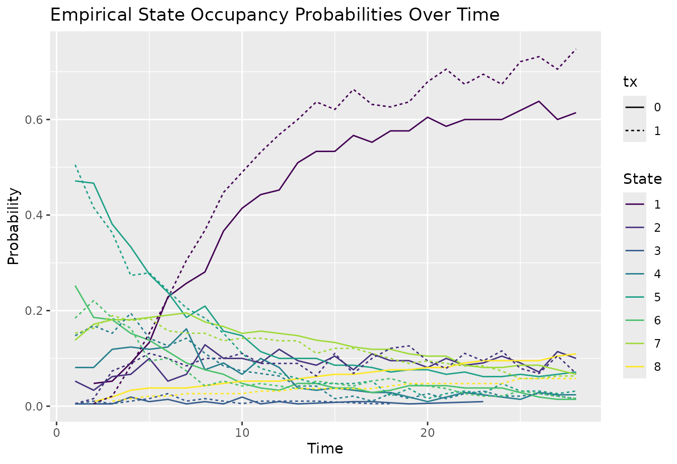
Fit a transition model
Both models below predict the state on each day, y, from
treatment, the previous day’s state, and a restricted cubic spline in
time with four knots, rcs(time, 4), which lets transition
probabilities change smoothly over follow-up. The models assume
proportional odds: each covariate shifts the odds of being in a
worse state by the same factor, whichever cut-point of the scale we look
at.
The formula syntax follows each backend. VGAM needs an ordered-factor
response and a cumulative() family, where
reverse = TRUE models the odds of worse (higher) states and
parallel = TRUE requests proportional odds. The rms model
needs a datadist object, which rms uses to summarize
predictors. The opt_method, scale, and
maxit arguments help rms::orm() converge
reliably.
In both wrappers, id_var = "id" tells mostr which rows
belong to the same patient. mostr uses it to compute standard errors
that account for repeated observations of the same patient, and it
stores the patient data needed later to estimate SOPs and their
confidence intervals.
fit_vglm <- vglm_markov(
  ordered(y) ~ tx + rcs(time, 4) + yprev,
  family = cumulative(reverse = TRUE, parallel = TRUE),
  data = model_data,
  id_var = "id"
)

dd <- datadist(model_data)
options(datadist = "dd")

fit_orm <- orm_markov(
  y ~ tx + rcs(time, 4) + yprev,
  data = model_data,
  id_var = "id",
  opt_method = "LM",
  scale = TRUE,
  maxit = 100
)

summary(fit_vglm)
Show output
#> Robust (Sandwich) Covariance Estimation for vglm
#> ================================================
#>
#> Call:
#> vglm_markov(formula = ordered(y) ~ tx + rcs(time, 4) + yprev,
#>     family = cumulative(reverse = TRUE, parallel = TRUE), data = model_data,
#>     id_var = "id")
#>
#> Number of observations: 10681
#> Bread: observed
#> HC type: HC0
#> Number of clusters: 400
#> Cluster adjustment: applied (n/(n-1))
#> Combined adjustment factor: 1.00251
#>
#> Coefficients (Robust SE):
#>                     Estimate Std. Error z value   Pr(>|z|)
#> (Intercept):1       -1.09132    0.11729  -9.304  1.350e-20 ***
#> (Intercept):2       -5.67529    0.29424 -19.288  6.739e-83 ***
#> (Intercept):3       -5.91091    0.29608 -19.964  1.137e-88 ***
#> (Intercept):4       -8.06245    0.29396 -27.427 1.294e-165 ***
#> (Intercept):5      -12.15511    0.31284 -38.854  0.000e+00 ***
#> (Intercept):6      -15.73679    0.33922 -46.391  0.000e+00 ***
#> (Intercept):7      -22.51763    0.39513 -56.989  0.000e+00 ***
#> tx                  -0.21232    0.05378  -3.948  7.882e-05 ***
#> rcs(time, 4)time    -0.16003    0.01654  -9.676  3.827e-22 ***
#> rcs(time, 4)time'    0.49286    0.05488   8.980  2.709e-19 ***
#> rcs(time, 4)time''  -1.28578    0.15615  -8.234  1.804e-16 ***
#> yprev2               0.09432    0.10841   0.870  3.843e-01
#> yprev3               6.10733    0.39938  15.292  8.622e-53 ***
#> yprev4               7.39295    0.28029  26.376 2.565e-153 ***
#> yprev5              10.13797    0.28470  35.609 1.011e-277 ***
#> yprev6              14.34958    0.31010  46.275  0.000e+00 ***
#> yprev7              19.70024    0.34290  57.451  0.000e+00 ***
#> ---
#> Signif. codes:  0 '***' 0.001 '**' 0.01 '*' 0.05 '.' 0.1 ' ' 1
#>
#> Model fit:
#>   deviance: 11449
#>   loglikelihood: -5724
fit_ormShow output
#> Logistic (Proportional Odds) Ordinal Regression Model
#>
#> rms::orm(formula = y ~ tx + rcs(time, 4) + yprev, data = model_data,
#>     opt_method = "LM", scale = TRUE, maxit = 100, x = TRUE, y = TRUE)
#>
#>
#> Frequencies of Responses
#>
#>    1    2    3    4    5    6    7    8
#> 5186  987   55  695 1557  752 1415   34
#>
#>                           Model Likelihood               Discrimination    Rank Discrim.
#>                                 Ratio Test                      Indexes          Indexes
#> Obs           10681    LR chi2    21222.55    R2                  0.905    rho     0.876
#> ESS          9385.4    d.f.             10    R2(10,10681)        0.863    Dxy     0.889
#> Distinct Y        8    Pr(> chi2)  <0.0001    R2(10,9385.4)       0.896
#> Cluster on  cluster                           |Pr(Y>=median)-0.5| 0.435
#> Clusters        400
#> Median Y          2
#> max |deriv|   3e-05
#>
#>         Coef     S.E.   Wald Z Pr(>|Z|)
#> y>=2     -1.0913 0.1173  -9.30 <0.0001
#> y>=3     -5.6753 0.2942 -19.29 <0.0001
#> y>=4     -5.9109 0.2961 -19.96 <0.0001
#> y>=5     -8.0624 0.2940 -27.43 <0.0001
#> y>=6    -12.1551 0.3128 -38.85 <0.0001
#> y>=7    -15.7368 0.3392 -46.39 <0.0001
#> y>=8    -22.5176 0.3951 -56.99 <0.0001
#> tx       -0.2123 0.0538  -3.95 <0.0001
#> time     -0.1600 0.0165  -9.68 <0.0001
#> time'     0.4929 0.0549   8.98 <0.0001
#> time''   -1.2858 0.1561  -8.23 <0.0001
#> yprev=2   0.0943 0.1084   0.87 0.3843
#> yprev=3   6.1073 0.3994  15.29 <0.0001
#> yprev=4   7.3929 0.2803  26.38 <0.0001
#> yprev=5  10.1380 0.2847  35.61 <0.0001
#> yprev=6  14.3496 0.3101  46.27 <0.0001
#> yprev=7  19.7002 0.3429  57.45 <0.0001
The two fits describe the same model, so their coefficients agree.
The tx coefficient is the log odds ratio for treatment; a
negative value means that treated patients tend to move to better
states. Its estimate should be close to the simulated value, \(\log(0.8) \approx -0.22\).
Estimate state occupancy probabilities
avg_sops() answers the question: what would the
probability of each state be on each day if every patient in the trial
had received control, and if every patient had received treatment?
It does so in three steps:
- For each patient, it sets
txto 0, starts from that patient’s observed state before day 1, and applies the model’s one-day transition probabilities day after day to obtain the patient’s SOPs. - It repeats the calculation with
txset to 1. - It averages the patient-level SOPs within each arm.
Because both arms are averaged over the same patients, differences between them reflect the treatment rather than differences in who was randomized to each arm.
The main arguments are:
-
variables = list(tx = c(0, 1)): the treatment values to compare; -
times: the days for which to report SOPs; -
y_levels: the states in the order used by the model; -
absorb: the absorbing state, so that patients who die stay dead.
inferences() then adds standard errors and 95%
confidence intervals. method = "delta" computes them
analytically, which is fast and needs no random draws.
vcov = "unconditional" makes the intervals account both for
uncertainty in the model coefficients and for the particular patients
who happened to enroll. See
vignette("analytical-confidence-intervals") for details and
alternatives.
sop_vglm <- avg_sops(
  fit_vglm,
  variables = list(tx = c(0, 1)),
  times = seq_len(FOLLOW_UP),
  y_levels = factor(STATE_LEVELS, levels = STATE_LEVELS),
  absorb = ABSORB
) |>
  inferences(
    method = "delta",
    vcov = "unconditional"
  )

sop_orm <- avg_sops(
  fit_orm,
  variables = list(tx = c(0, 1)),
  times = seq_len(FOLLOW_UP),
  y_levels = fit_orm$yunique,
  absorb = ABSORB
) |>
  inferences(
    method = "delta",
    vcov = "unconditional"
  )

combined_sops <- rbind(
  data.frame(backend = "VGAM vglm", as.data.frame(sop_vglm)),
  data.frame(backend = "rms orm", as.data.frame(sop_orm))
)
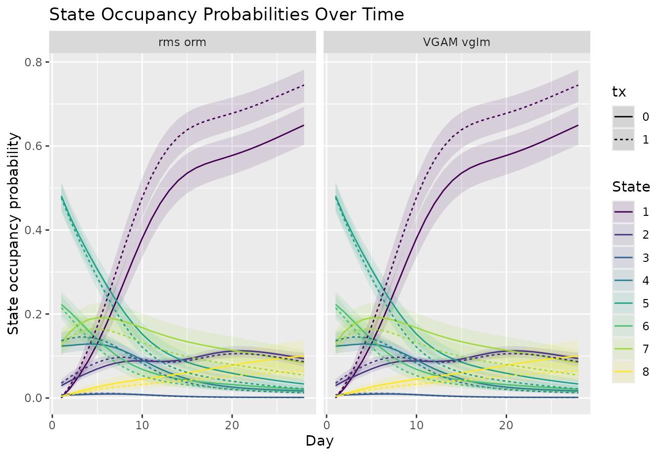
The result has one row per day, state, and treatment value, with the
estimated probability in estimate and its confidence limits
in conf.low and conf.high. Plotting both
backends side by side confirms that they agree.
plot_sops(
  combined_sops,
  geom = "line",
  linetype_var = "tx",
  facet_var = c("backend")
) +
  labs(
    x = "Day",
    y = "State occupancy probability"
  )
How the probabilities are calculated
This section states the calculation behind avg_sops()
precisely. You can skip it on a first reading.
Let \(i = 1,\ldots,n\) index patients and \(t = 1,\ldots,d\) index follow-up days. Patient \(i\)’s state on day \(t\) is \(Y_{it}\), one of \(K\) ordered states numbered \(1,\ldots,K\), and \(Y_{i0}\) is the observed state before the first day. The vector \(\mathbf{x}_{it}\) holds treatment, time, and any other covariates on day \(t\), and \(\mathbf{x}_{i,1:t} = (\mathbf{x}_{i1},\ldots,\mathbf{x}_{it})\) holds their values up to day \(t\). The SOP for state \(l\) is
\[ S_{it}(l) = \Pr(Y_{it} = l \mid \mathbf{x}_{i,1:t}, Y_{i0}). \]
The fitted model supplies the transition probability: the probability of moving from state \(k\) on day \(t - 1\) to state \(l\) on day \(t\),
\[ T_{it}(l \mid k) = \Pr(Y_{it} = l \mid Y_{i,t-1} = k, \mathbf{x}_{it}). \]
This is a first-order Markov model: given today’s state, tomorrow’s state does not depend on earlier states. For an absorbing state \(k\) we do not use the model at all but set \(T_{it}(l \mid k) = 1\) if \(l = k\) and \(0\) otherwise, so a patient who has died stays dead.
To obtain the SOPs, add up the probability of arriving in state \(l\) from each possible previous state:
\[ S_{it}(l) = \sum_{k=1}^{K} S_{i,t-1}(k)\, T_{it}(l \mid k), \qquad t = 1,\ldots,d, \]
starting from \(S_{i0}(l) = 1\) for the observed starting state \(l = Y_{i0}\) and \(0\) for every other state. In matrix form, if \(\mathbf{s}_{it}\) is the row vector of SOPs and \(\mathbf{P}_{it}\) is the \(K \times K\) matrix with \(T_{it}(l \mid k)\) in row \(k\) and column \(l\), each day’s update is \(\mathbf{s}_{it} = \mathbf{s}_{i,t-1}\mathbf{P}_{it}\). mostr performs this update for all patients at once and never has to predict transitions out of an absorbing state; probability already in such a state is simply carried forward.
Finally, write \(S_{it}(l; z)\) for
the SOP calculated with treatment set to \(z\) on every day. The arm-specific SOP
reported by avg_sops() is the average over patients,
\[ \bar{S}_t(l; z) = \frac{1}{n} \sum_{i=1}^n S_{it}(l; z). \]
Check the model against the data
SOPs are only as trustworthy as the transition model behind them. mostr’s diagnostic plots compute a summary once from the observed trajectories and once from the fitted model, so that you can compare the two side by side. Clear disagreements suggest that the model misses a feature of the data, for example a time trend, an interaction, or dependence on states before the previous day.
Correlation between days
plot_correlation() shows the Spearman rank correlation
between patients’ states on every pair of days. The first plot uses the
observed data; the second uses the correlations implied by the model.
Both should show similar patterns: high correlation between nearby days
that weakens as days get further apart. By default, each plot chooses
its own color scale, so we set fill_limits = c(0, 1) to
give both plots the same scale. If any correlation were negative, we
would use c(-1, 1) instead, because values outside the
limits are shown in grey.
ec <- plot_correlation(
  fill_limits = c(0, 1),
  show_values = FALSE,
  raw_data,
  id_var = "id",
  time_var = "time",
  y_var = "y"
)

mc <- plot_correlation(
  fill_limits = c(0, 1),
  show_values = FALSE,
  fit_orm,
  id_var = "id",
  time_var = "time",
  y_var = "y",
  times = seq_len(FOLLOW_UP),
  y_levels = fit_orm$yunique,
  absorb = ABSORB
)

ec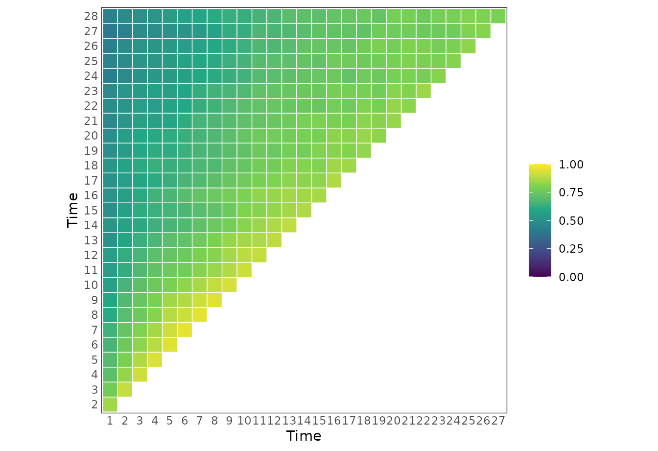
mc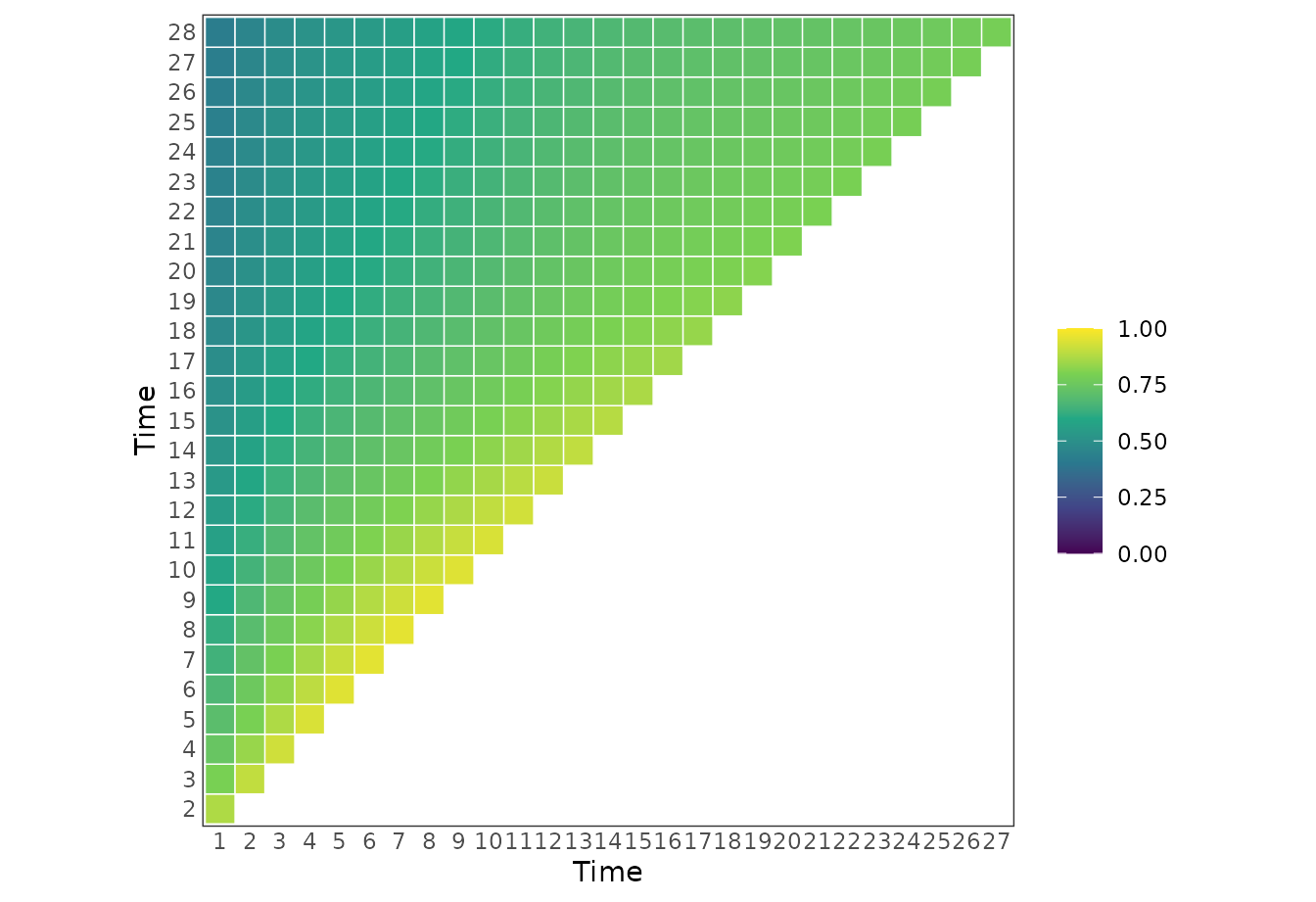
Transitions between states
plot_transitions() draws, for selected days, a heatmap
of the proportion of patients who move from each previous state (rows)
to each current state (columns). Comparing the observed and model-based
heatmaps shows whether the model reproduces how patients move between
states over follow-up. We show at most sixteen evenly spaced days so
each panel stays readable.
diagnostic_times <- unique(round(seq(1, FOLLOW_UP, length.out = min(16L, FOLLOW_UP))))

et <- plot_transitions(
  raw_data,
  id_var = "id",
  time_var = "time",
  y_var = "y",
  times = diagnostic_times,
  show_values = FALSE
)

mt <- plot_transitions(
  fit_orm,
  id_var = "id",
  time_var = "time",
  y_var = "y",
  times = diagnostic_times,
  y_levels = fit_orm$yunique,
  absorb = ABSORB,
  show_values = FALSE
)

et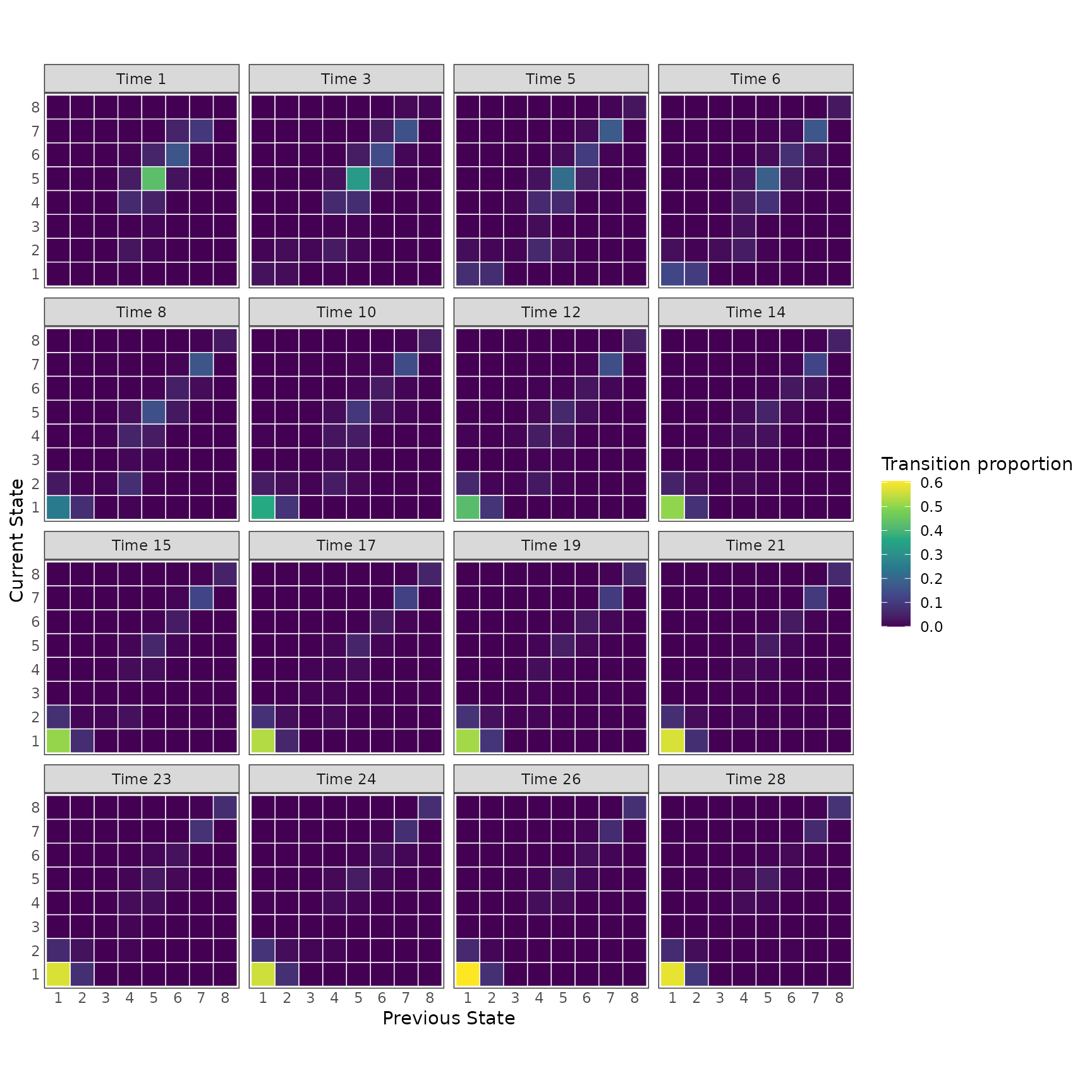
mt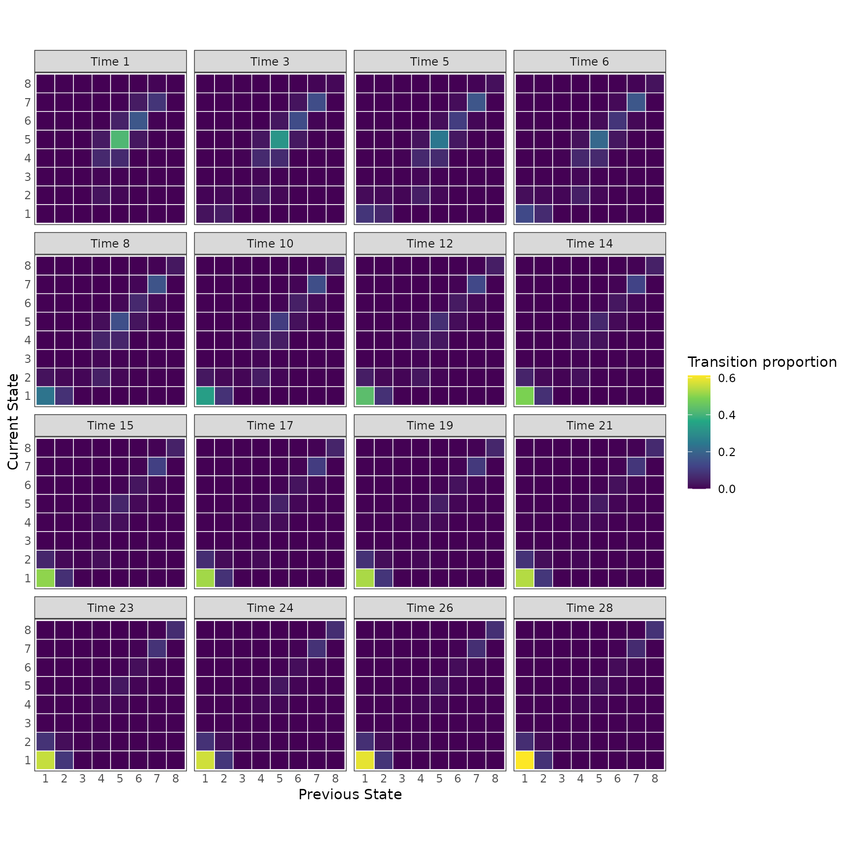
With comparison = "difference", the same function shows
how treatment changes the model-based transition proportions: each tile
is the proportion under tx = 1 minus the proportion under
tx = 0.
td <- plot_transitions(
  fit_orm,
  comparison = "difference",
  variables = list(tx = c(0, 1)),
  id_var = "id",
  time_var = "time",
  y_var = "y",
  times = diagnostic_times,
  y_levels = fit_orm$yunique,
  absorb = ABSORB,
  show_values = FALSE
)
td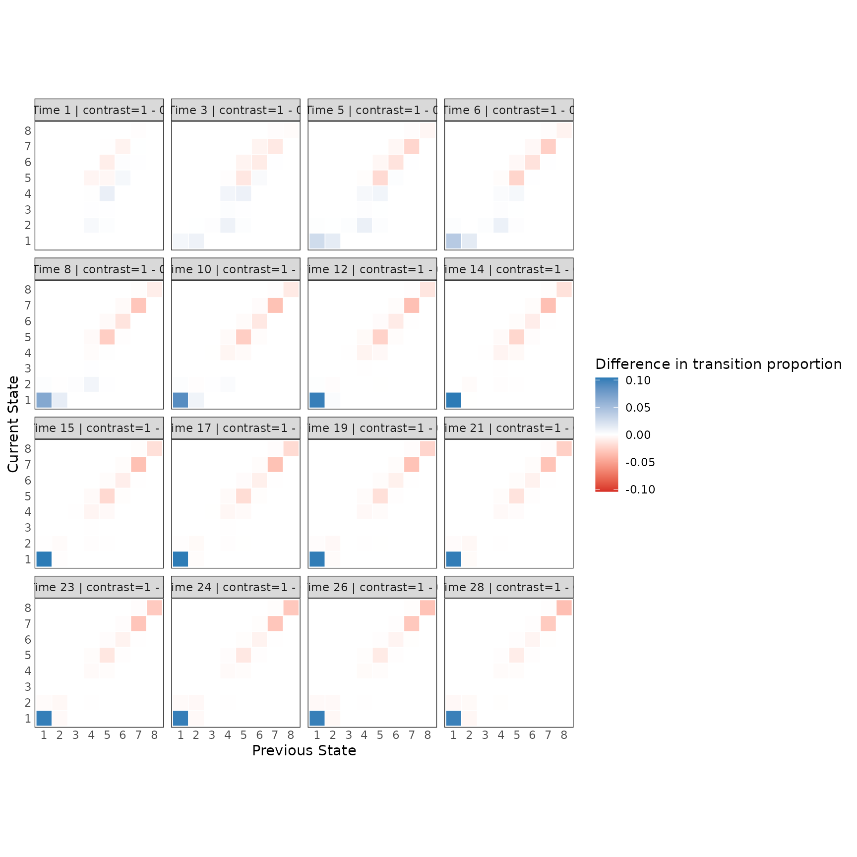
How correlation decays with time
plot_variogram() condenses the correlation matrix into a
single curve: the correlation between two days plotted against the
number of days between them. If the observed correlations fall off more
slowly than the model’s, patients’ earlier history matters more than a
first-order model allows, and a second-order model (see
vignette("second-order-orm-sops")) may fit better.
plot_variogram(
  raw_data,
  id_var = "id",
  time_var = "time",
  y_var = "y"
) +
  coord_cartesian(ylim = c(0, 1))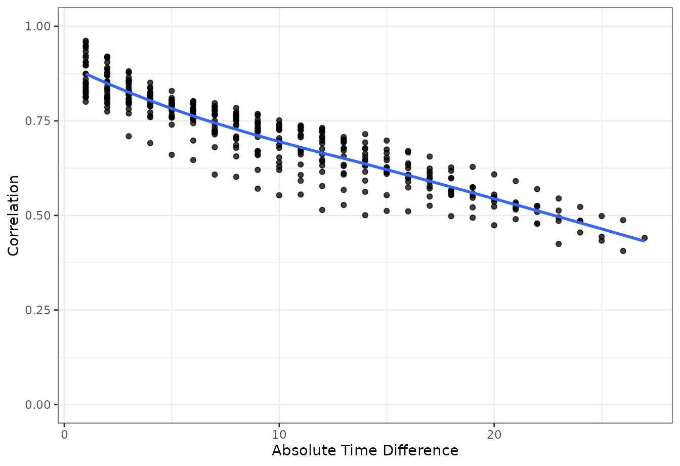
plot_variogram(
  fit_orm,
  id_var = "id",
  time_var = "time",
  y_var = "y",
  times = seq_len(FOLLOW_UP),
  y_levels = fit_orm$yunique,
  absorb = ABSORB
) +
  coord_cartesian(ylim = c(0, 1))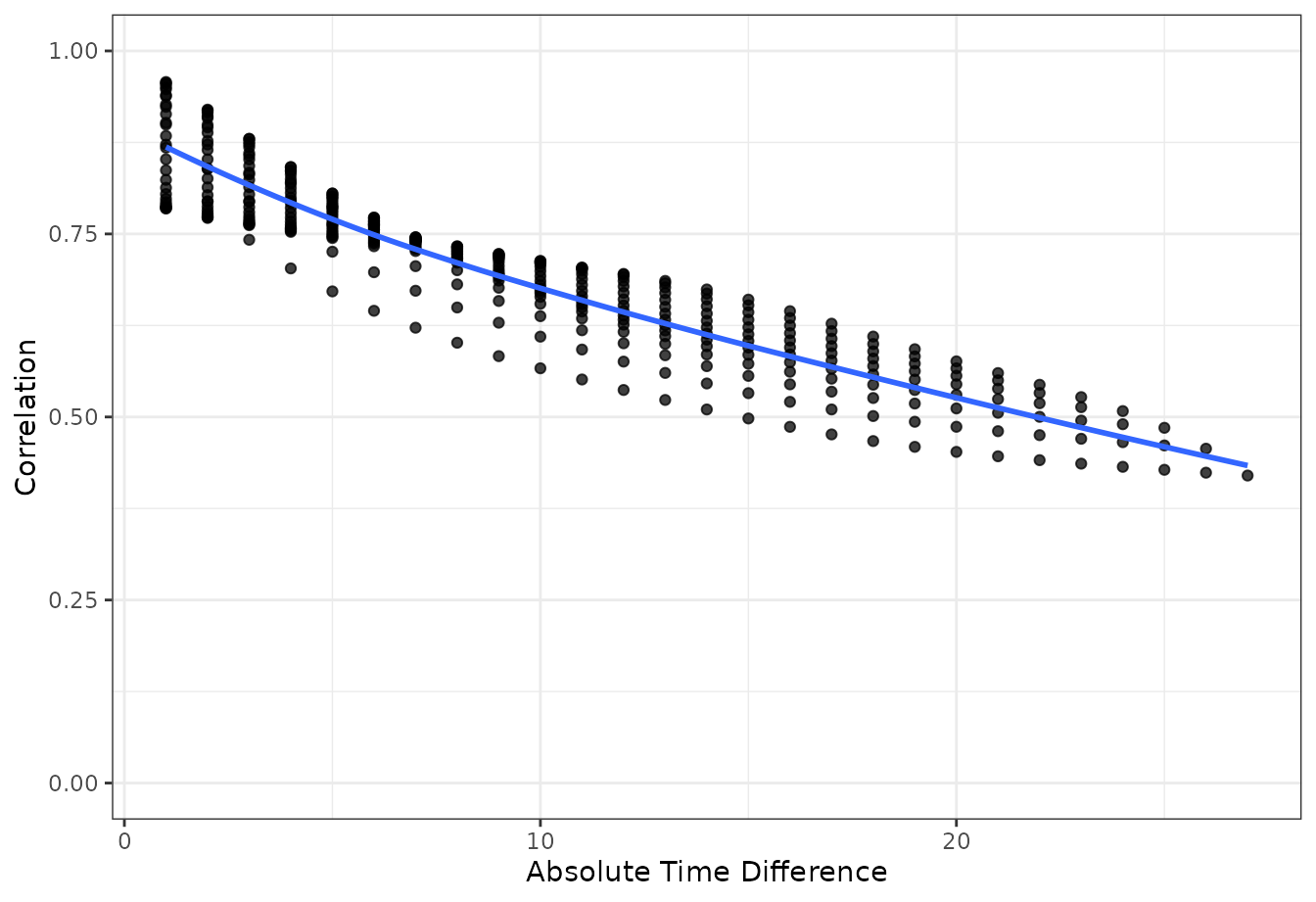
Where to go next
-
vignette("analytical-confidence-intervals")explains the confidence intervals used here and how to compare arms directly withavg_comparisons(). -
vignette("partial-po-vglm-sops"),vignette("second-order-orm-sops"),vignette("factor-time-orm-sops"), andvignette("many-levels-previous-state-spline")show other model specifications. -
vignette("mvn-vs-bootstrap-orm-sops"),vignette("fractional-weighted-bootstrap-sops"), andvignette("bayesian-rmsb-sops")show simulation-based, resampling-based, and Bayesian uncertainty.