blrm_markov() fits a Bayesian transition model with
rmsb::blrm(), which samples from the posterior distribution
of the coefficients using Stan. The state occupancy probabilities (SOPs)
and comparisons calculated from it carry posterior uncertainty directly:
mostr computes the SOPs for each posterior draw of the coefficients and
summarizes the results. No separate inferences() step is
needed.
This article fits a Bayesian model in which the effect of time may depart from proportional odds, computes posterior SOPs, and checks the model against the data.
Fitting the model takes a while, so the model-based code below runs
only when the environment variable
MOSTR_RUN_BAYESIAN_VIGNETTE is "true" and the
rmsb package is installed. The example uses few MCMC iterations to keep
running time short; a real analysis needs more iterations and a check of
sampling diagnostics.
Data
We simulate 200 patients over 14 days with
sim_markov("actt2"), which uses the eight-state NIAID scale
described in vignette("full-po-sops"), and plot the
observed proportion of patients in each state.
library(mostr)
library(ggplot2)
library(rms)
library(rmsb)

N_PATIENTS <- 200
FOLLOW_UP <- 14
SEED <- 20260601
STATE_LEVELS <- as.character(1:8)
ABSORB <- "8"
SOP_DRAWS <- 200

raw_data <- sim_markov(
  "actt2",
  n_patients = N_PATIENTS,
  follow_up_time = FOLLOW_UP,
  treatment_effect = -0.03,
  seed = SEED
)

model_data <- prepare_markov_data(raw_data, absorbing_state = 8)
plot_sops(raw_data)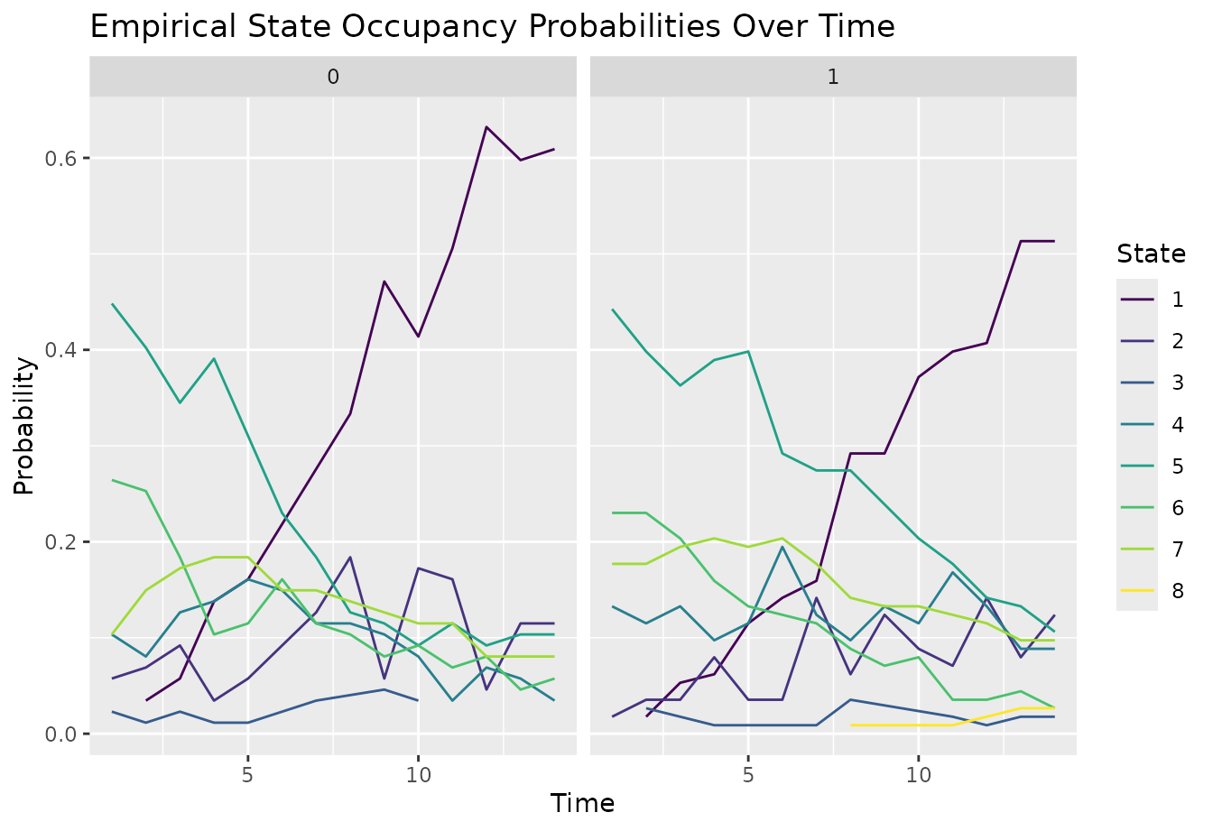
Fit the model
The formula includes the previous state and a treatment-by-time interaction, with time modeled by a restricted cubic spline. Two further arguments relax proportional odds for time:
-
ppo = ~ timeallows the effect of time to differ between cut-points of the ordinal scale; -
cppo = function(y) as.numeric(y)constrains that difference to change linearly with the state number, so it adds only one coefficient.
cluster(id) adds a random effect for each patient, which
allows for patient-level differences not explained by the
covariates.
dd <- rms::datadist(model_data)
options(datadist = "dd")

fit_blrm <- blrm_markov(
  y ~ yprev + rms::rcs(time, 4) * tx + cluster(id),
  ppo = ~ time,
  cppo = function(y) as.numeric(y),
  data = model_data,
  id_var = "id",
  iter = 300,
  warmup = 150,
  chains = 2,
  method = "sampling",
  refresh = 0,
  seed = SEED
)
fit_blrm
Show output
#> Bayesian Constrained Partial Proportional Odds Ordinal Logistic Model
#>
#> Dirichlet Priors With Concentration Parameter 0.278 for Intercepts
#>
#> rmsb::blrm(formula = y ~ yprev + rms::rcs(time, 4) * tx + cluster(id),
#>     ppo = ~time, cppo = function (y)
#>     as.numeric(y), data = model_data, iter = 300, warmup = 150,
#>     chains = 2, method = "sampling", refresh = 0, seed = SEED,
#>     x = TRUE, y = TRUE)
#>
#>
#> Frequencies of Responses
#>
#>   1   2   3   4   5   6   7   8
#> 764 241  37 315 699 328 404   3
#>
#>                                            Mixed Calibration/               Discrimination               Rank Discrim.
#>                                        Discrimination Indexes                      Indexes                     Indexes
#> Obs                            2791    B 0.036 [0.036, 0.036]    g     7.678 [7.216, 8.14]    C   0.957 [0.956, 0.958]
#> Draws                           300                              gp   0.377 [0.366, 0.387]    Dxy 0.914 [0.913, 0.916]
#> Chains                            2                              EV   0.815 [0.781, 0.842]
#> Time                          37.6s                              v  46.544 [41.25, 52.382]
#> p                                13                              vp    0.162 [0.152, 0.17]
#> Cluster on                       id
#> Clusters                        200
#> sigma gamma 0.2305 [0.0062, 0.4647]
#>
#>             Mean Beta Median Beta S.E.   Lower    Upper    Pr(Beta>0) Symmetry
#> y>=2          0.0676    0.0878    0.4359  -0.8599   0.8780 0.5700     0.95
#> y>=3         -3.9132   -3.9111    0.5158  -4.9534  -3.0545 0.0000     1.05
#> y>=4         -4.2910   -4.3047    0.5048  -5.2890  -3.3775 0.0000     0.99
#> y>=5         -6.6500   -6.6405    0.5009  -7.6184  -5.7286 0.0000     0.98
#> y>=6        -10.9870  -10.9599    0.5221 -12.0181 -10.0327 0.0000     0.97
#> y>=7        -15.0663  -15.0224    0.5746 -16.0763 -13.9173 0.0000     0.91
#> y>=8        -22.9542  -22.9267    0.8672 -24.7643 -21.3647 0.0000     0.92
#> yprev=2      -0.1962   -0.2019    0.2617  -0.7177   0.3026 0.2233     0.93
#> yprev=3       5.5798    5.5573    0.5127   4.5570   6.5008 1.0000     1.02
#> yprev=4       6.3709    6.3473    0.4222   5.6262   7.2386 1.0000     1.16
#> yprev=5       9.5156    9.4690    0.4321   8.8064  10.4009 1.0000     1.27
#> yprev=6      13.7417   13.7331    0.4617  12.9909  14.6345 1.0000     1.47
#> yprev=7      19.3860   19.3496    0.5800  18.2120  20.4816 1.0000     1.01
#> time         -0.4101   -0.4086    0.1013  -0.5876  -0.2133 0.0000     1.13
#> time'         0.6119    0.6110    0.2853   0.0911   1.1678 0.9867     1.05
#> time''       -0.9530   -0.9331    0.7259  -2.2660   0.5352 0.0900     0.95
#> tx           -0.2563   -0.2572    0.3720  -0.9029   0.4756 0.2567     0.95
#> time * tx     0.1092    0.1160    0.1200  -0.1011   0.3461 0.8067     0.94
#> time' * tx   -0.2012   -0.2095    0.3929  -1.0247   0.4734 0.2967     1.02
#> time'' * tx   0.2733    0.2587    0.9963  -1.8149   2.1109 0.6300     1.00
#> time x f(y)   0.0011    0.0010    0.0083  -0.0129   0.0179 0.5567     1.12
Posterior SOPs
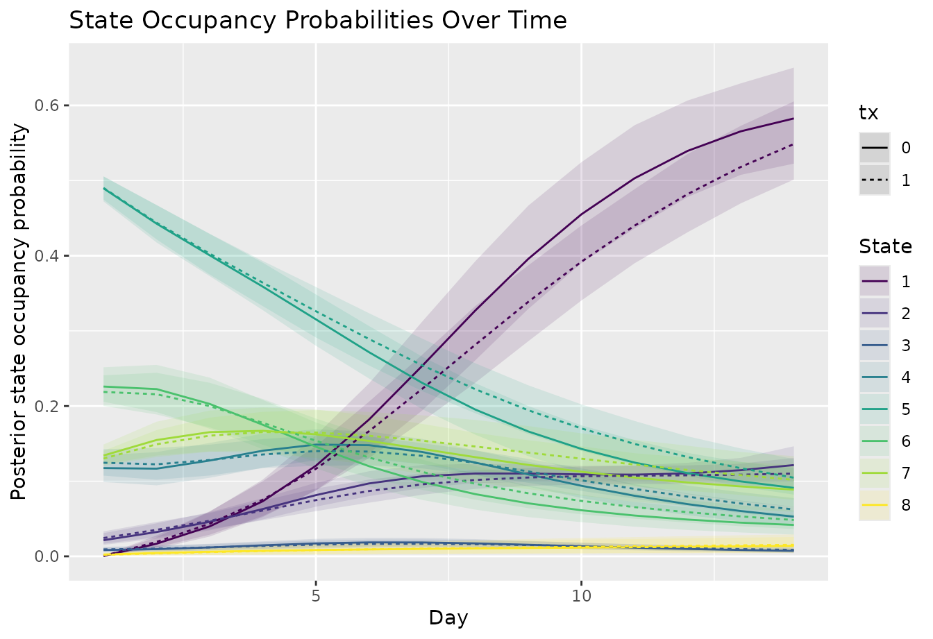
For Bayesian fits, avg_sops() computes the SOPs for each
posterior draw and then summarizes them. The arguments specific to
Bayesian fits are:
-
n_draws = NULLuses all stored posterior draws; a number uses a random subset of that size, selected reproducibly withseed; -
include_re = TRUEincludes each patient’s estimated random effect in the predictions; -
posterior_summary = "mean"reports the posterior mean. Unlike the median, the means across states always add up to 1; -
conf_level = 0.90requests 90% posterior intervals; -
return_draws = TRUEkeeps the draw-level SOPs, whichget_draws()extracts.
Averaging over patients for every posterior draw can need a lot of
memory. options(mostr.blrm_avg_chunk_size = 100) processes
the draws in groups of 100 to limit it.
options(mostr.blrm_avg_chunk_size = 100)

sop_blrm <- avg_sops(
  fit_blrm,
  variables = list(tx = c(0, 1)),
  times = seq_len(FOLLOW_UP),
  y_levels = fit_blrm$ylevels,
  absorb = ABSORB,
  include_re = TRUE,
  n_draws = NULL,
  seed = SEED,
  posterior_summary = "mean",
  conf_level = 0.90,
  return_draws = TRUE
)

head(sop_blrm)
#> time state tx estimate conf.low conf.high std.error
#> 1 1 1 0 0.0005112346 0.0001758787 0.001030758 0.0002500782
#> 2 2 1 0 0.0168236591 0.0100423026 0.025332409 0.0045761444
#> 3 3 1 0 0.0398881774 0.0263646596 0.059409589 0.0095991035
#> 4 4 1 0 0.0733599974 0.0522980274 0.102125366 0.0153235817
#> 5 5 1 0 0.1206003871 0.0878444301 0.161077294 0.0217035762
#> 6 6 1 0 0.1820603438 0.1372658117 0.230068021 0.0284179613
plot_sops(
  sop_blrm,
  geom = "line",
  facet_var = NULL,
  linetype_var = "tx"
) +
  labs(
    x = "Day",
    y = "Posterior state occupancy probability"
  )
Check the model against the data
As in vignette("full-po-sops"), each diagnostic is
computed once from the observed trajectories and once from the fitted
model. For Bayesian fits, the model-based summary is calculated
separately for each posterior draw and only then summarized across
draws; seed makes the choice of draws reproducible. The
transition heatmaps use at most sixteen evenly spaced days.
diagnostic_times <- unique(round(seq(1, FOLLOW_UP, length.out = min(16L, FOLLOW_UP))))

plot_transitions(
  raw_data,
  times = diagnostic_times,
  y_levels = STATE_LEVELS,
  show_values = FALSE
) +
  labs(title = "Observed transition proportions")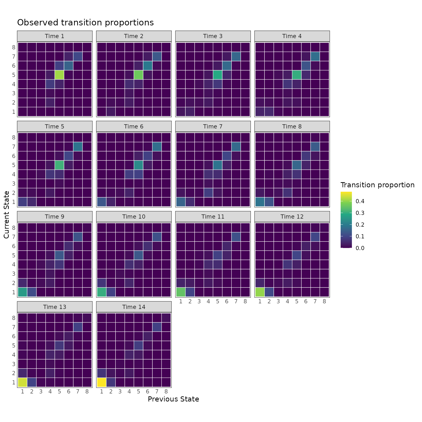
plot_transitions(
  fit_blrm,
  times = diagnostic_times,
  y_levels = fit_blrm$ylevels,
  absorb = ABSORB,
  seed = SEED,
  show_values = FALSE
) +
  labs(title = "Model-based transition proportions")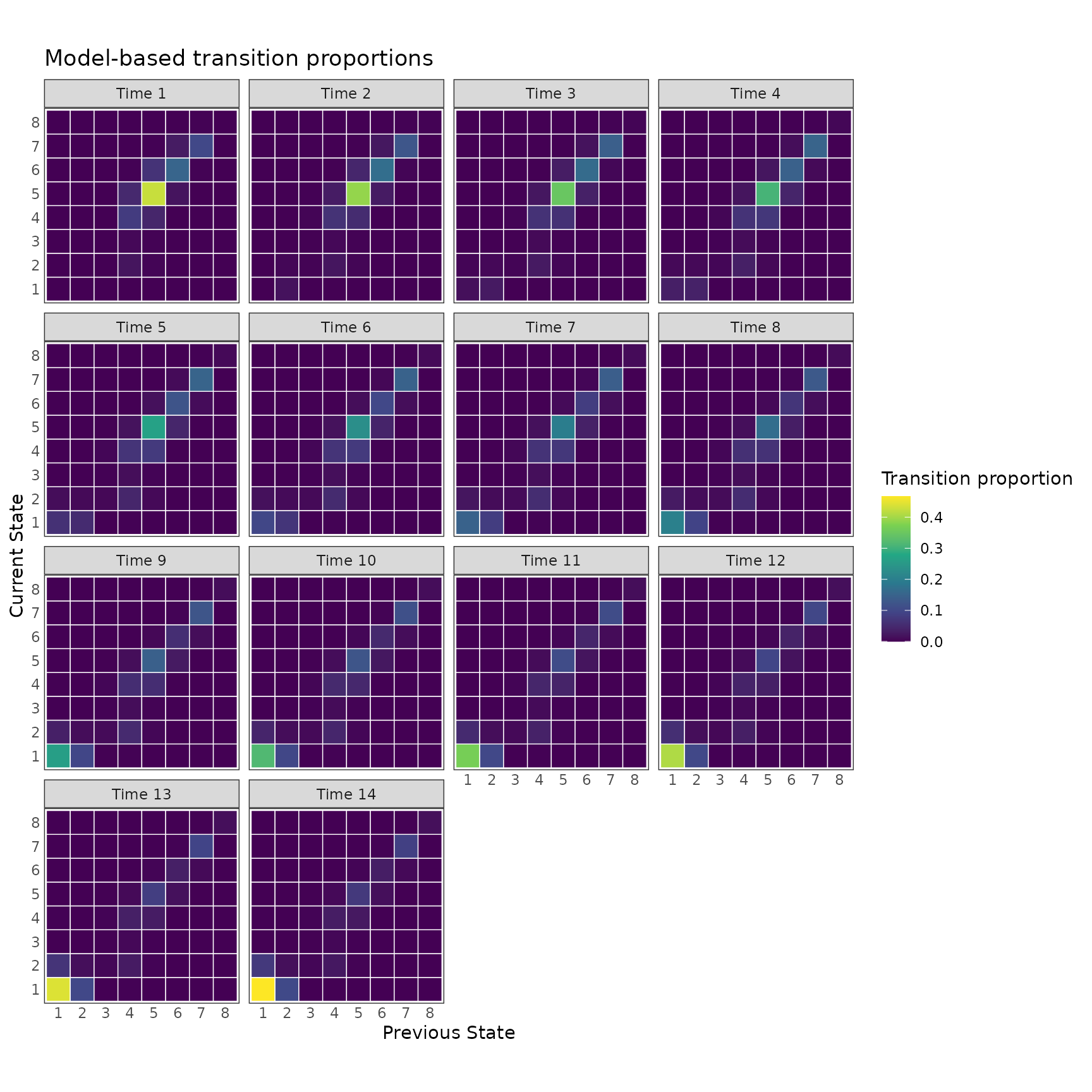
plot_correlation(
  fill_limits = c(0, 1),
  raw_data,
  times = seq_len(FOLLOW_UP),
  show_values = FALSE
) +
  labs(title = "Observed state correlations")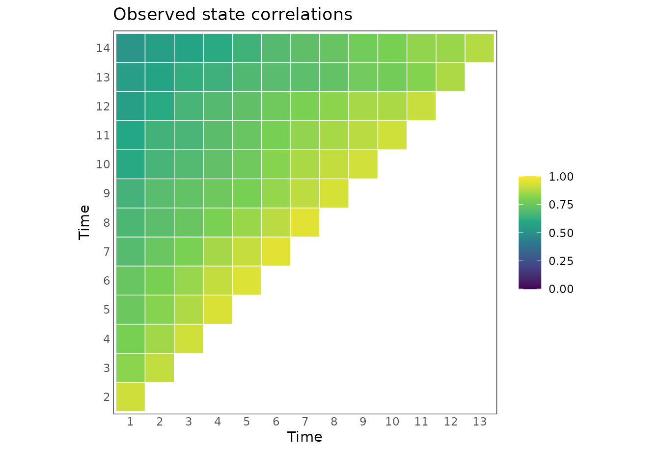
plot_correlation(
  fill_limits = c(0, 1),
  fit_blrm,
  times = seq_len(FOLLOW_UP),
  y_levels = fit_blrm$ylevels,
  absorb = ABSORB,
  seed = SEED,
  show_values = FALSE
) +
  labs(title = "Model-based state correlations")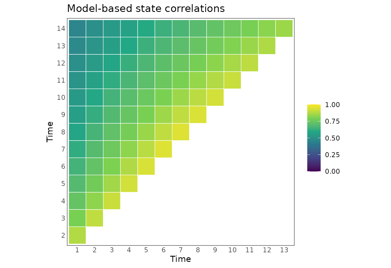
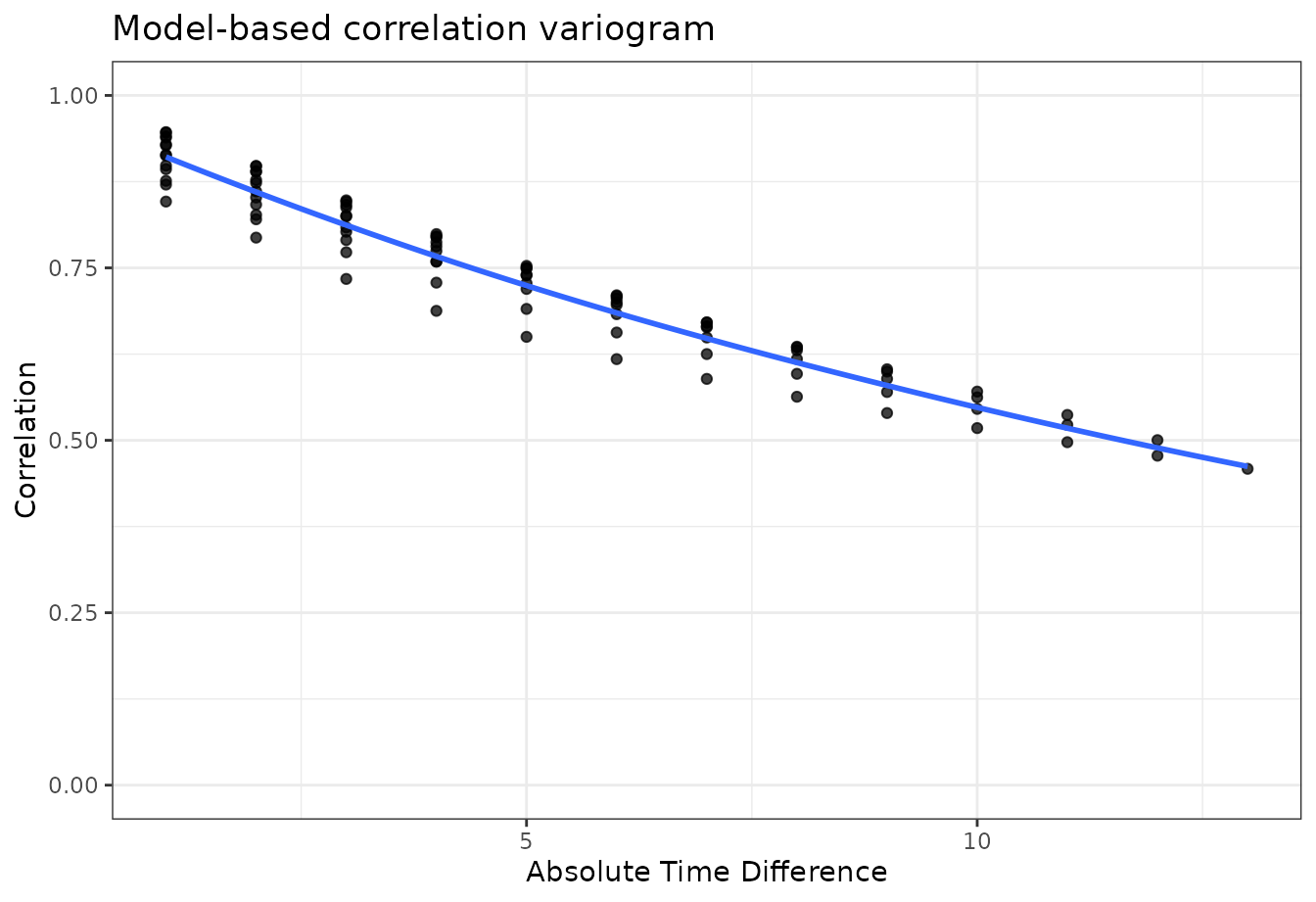
plot_variogram(
  raw_data,
  times = seq_len(FOLLOW_UP)
) +
  labs(title = "Observed correlation variogram")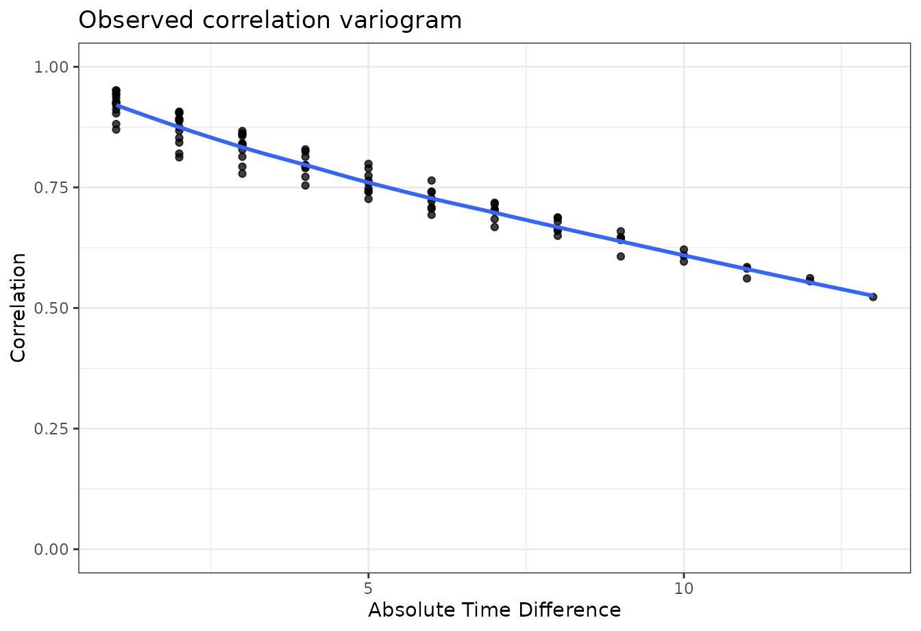
plot_variogram(
  fit_blrm,
  times = seq_len(FOLLOW_UP),
  y_levels = fit_blrm$ylevels,
  absorb = ABSORB,
  seed = SEED
) +
  labs(title = "Model-based correlation variogram")