Time as a Factor with orm_markov()

Many studies assess patients at a few scheduled visits rather than every day, for example on days 3, 7, 14, and 21. The state between visits is then unknown and cannot be reconstructed reliably. In this situation, a transition model can describe the change from one visit to the next, with each visit treated as a separate category of time.

This article shows how to

1. turn daily data into visit data and fit an orm_markov() model with time as a factor;
2. estimate state occupancy probabilities (SOPs) at each visit;
3. convert these to a calendar-day scale by interpolating between visits; and
4. compare the expected number of days spent in each state between arms.

Visit data

We simulate daily states for 220 patients with sim_markov("actt2"), which uses the eight-state NIAID scale described in vignette("full-po-sops"), and keep only days 3, 7, 14, and 21. The observed SOPs of the full daily data are shown for reference.

library(mostr)
library(ggplot2)
library(rms)

N_PATIENTS <- 220
SEED <- 20260531
VISIT_DAYS <- stats::setNames(c(3, 7, 14, 21), as.character(1:4))
STATE_LEVELS <- as.character(1:8)
ABSORB <- 8L

raw_data <- sim_markov(
  "actt2",
  n_patients = N_PATIENTS,
  treatment_effect = log(0.8),
  seed = SEED
)

plot_sops(raw_data, facet_var = NULL, linetype_var = "tx")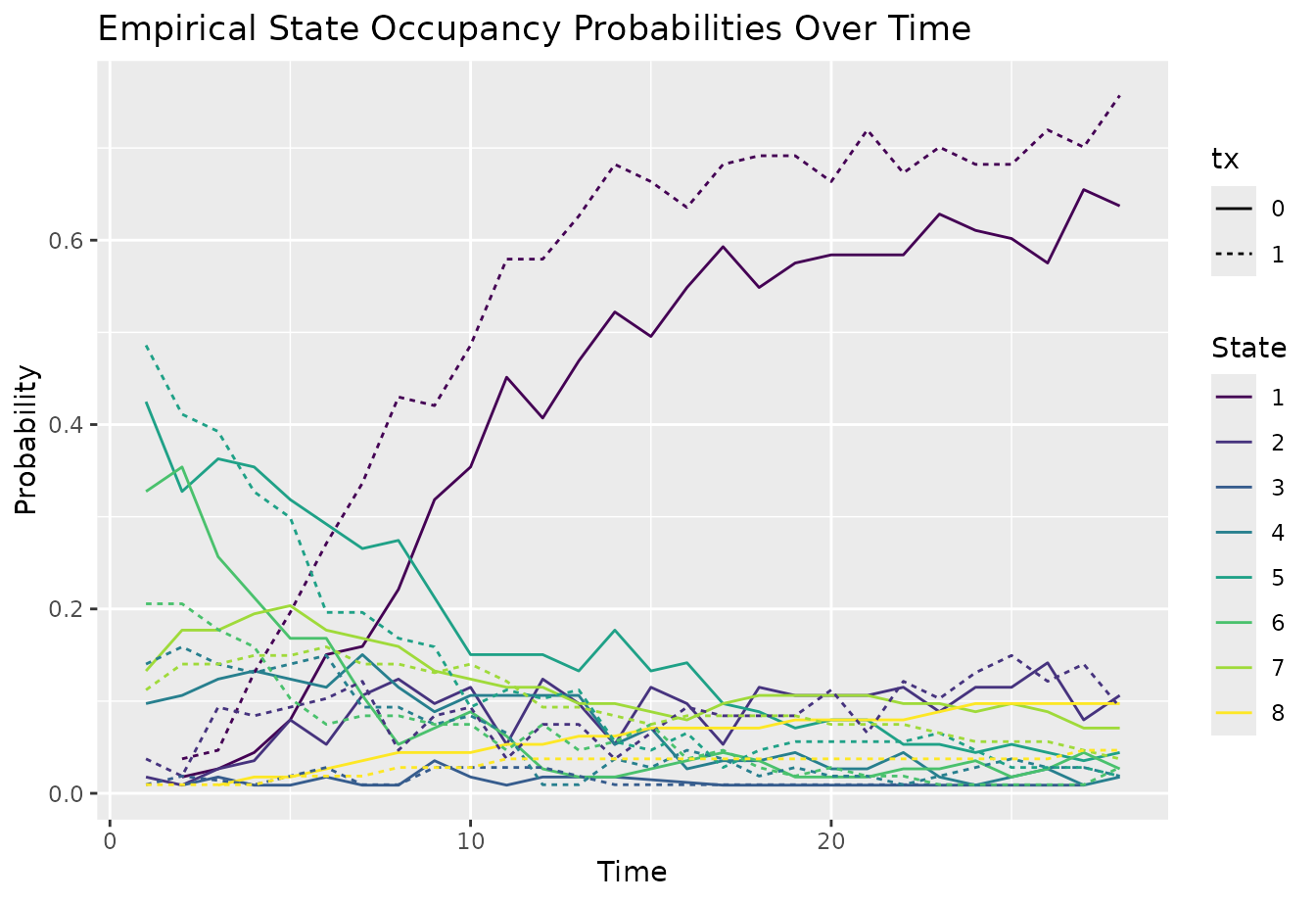

VISIT_DAYS links each visit number to its calendar day. To build the visit data, we

• keep the rows for the four visit days;
• recode time as a factor with levels "1" to "4" (the visit number), keeping the calendar day in visit_day;
• set yprev to the state at the previous visit rather than the previous day; and
• for the first visit, use the patient’s state before day 1 as yprev, so that every patient’s starting state is the same observed baseline state.

baseline_state <- raw_data[raw_data$time == 1, c("id", "yprev")]
names(baseline_state)[2] <- "baseline_yprev"

visit_data <- raw_data[
  raw_data$time %in% unname(VISIT_DAYS),
  c("id", "tx", "time", "y", "yprev")
]
visit_data <- merge(
  visit_data,
  baseline_state,
  by = "id",
  all.x = TRUE,
  sort = FALSE
)
visit_data <- visit_data[order(visit_data$id, visit_data$time), ]
visit_data$visit_day <- visit_data$time
visit_data$time <- factor(
  match(visit_data$visit_day, unname(VISIT_DAYS)),
  levels = seq_along(VISIT_DAYS),
  labels = names(VISIT_DAYS)
)
visit_data$yprev <- ave(
  visit_data$y,
  visit_data$id,
  FUN = function(y) c(NA_integer_, y[-length(y)])
)
first_visit <- !duplicated(visit_data$id)
visit_data$yprev[first_visit] <- visit_data$baseline_yprev[first_visit]
visit_data$baseline_yprev <- NULL

model_data <- prepare_markov_data(
  visit_data,
  absorbing_state = ABSORB,
  factor_previous = TRUE
)

head(model_data)

#>   id tx time y yprev visit_day
#> 1  1  0    1 4     5         3
#> 2  1  0    2 1     4         7
#> 3  1  0    3 1     1        14
#> 4  1  0    4 1     1        21
#> 5  2  1    1 5     5         3
#> 6  2  1    2 7     5         7

Fit the model and estimate SOPs at each visit

With time as a factor, the model estimates a separate effect for each visit, so the intervals between visits may differ in length without any assumption about how transition probabilities change from day to day.

mostr needs to know which visit is the first, because each patient’s starting state and covariates are taken from their row at that visit. For numeric time this defaults to 1; for factor time, set it explicitly with first_followup_time = "1". Likewise, pass the visit labels, not calendar days, to times in avg_sops(). The resulting SOPs refer to visits 1 to 4.

dd <- rms::datadist(model_data)
options(datadist = "dd")

fit_visit <- orm_markov(
  y ~ tx + time + yprev,
  data = model_data,
  id_var = "id",
  first_followup_time = "1",
  opt_method = "LM",
  scale = TRUE,
  maxit = 100
)

sop_visit <- avg_sops(
  fit_visit,
  variables = list(tx = c(0, 1)),
  times = names(VISIT_DAYS),
  y_levels = fit_visit$yunique,
  absorb = as.character(ABSORB)
) |>
  inferences(method = "delta", vcov = "unconditional")

head(sop_visit)

#>   time state tx   estimate   std.error   conf.low  conf.high
#> 1    1     1  0 0.06723135 0.009920164 0.05020841 0.08948209
#> 2    2     1  0 0.22963719 0.024237863 0.18559386 0.28053215
#> 3    3     1  0 0.48337960 0.036598252 0.41247371 0.55496110
#> 4    4     1  0 0.54893267 0.037668973 0.47456798 0.62117402
#> 5    1     2  0 0.06216972 0.009594324 0.04581601 0.08384782
#> 6    2     2  0 0.08727451 0.011765845 0.06680268 0.11325857

Interpolate to calendar days

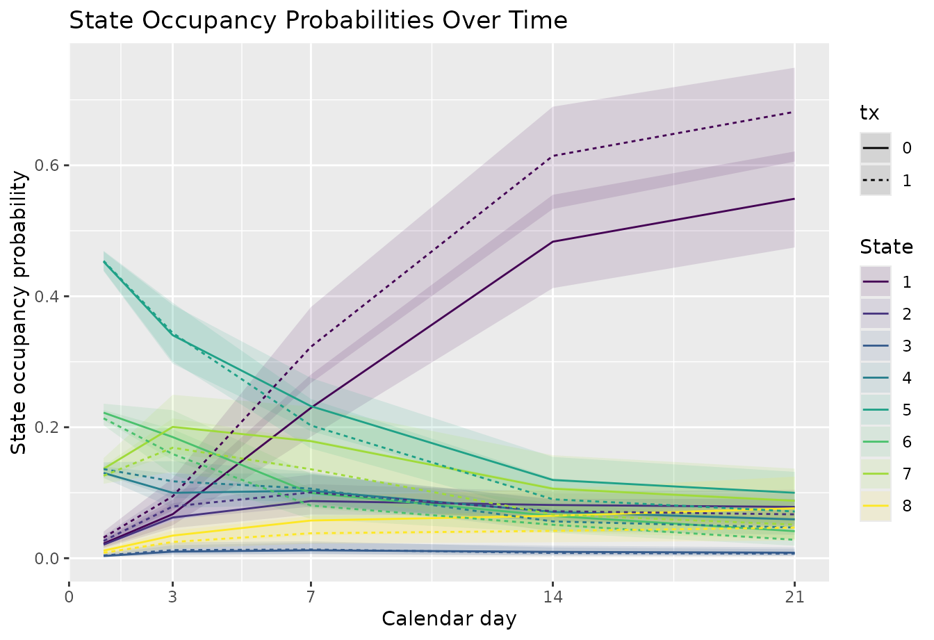
interpolate_sops() places the visit-scale SOPs on the calendar-day scale:

• time_map = VISIT_DAYS maps each visit label to its day;
• baseline_time = 0 adds the observed distribution of starting states (yprev at the first visit) as the SOPs on day 0;
• target_times = 1:21 requests every day from 1 to 21.

Between two known time points, each probability is interpolated linearly. The day-0 baseline anchors the interpolation for days 1 and 2, before the first visit, but is not itself part of the returned grid. Interpolated values are a convenient summary, not model predictions for the unobserved days.

sop_days <- interpolate_sops(
  sop_visit,
  time_map = VISIT_DAYS,
  target_times = 1:max(VISIT_DAYS),
  baseline_time = 0
)

plot_sops(
  sop_days,
  time_var = "time",
  geom = "line",
  facet_var = NULL,
  linetype_var = "tx"
) +
  scale_x_continuous(breaks = c(0, unname(VISIT_DAYS))) +
  labs(
    x = "Calendar day",
    y = "State occupancy probability"
  )

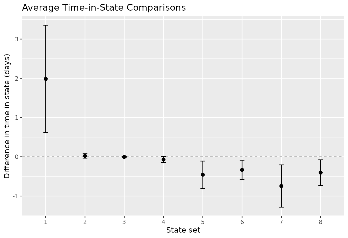
Compare time in each state

avg_comparisons() accepts the same time_map, target_times, and baseline_time arguments. With them, estimand = "time_in_state" measures the expected number of calendar days, rather than visits, spent in each state over days 1 to 21. time_unit = "days" labels the result. Each estimate is treated minus control.

cmp_days <- avg_comparisons(
  fit_visit,
  variables = list(tx = c(0, 1)),
  estimand = "time_in_state",
  state_sets = NULL,
  comparison = "difference",
  times = names(VISIT_DAYS),
  y_levels = fit_visit$yunique,
  absorb = as.character(ABSORB),
  time_map = VISIT_DAYS,
  target_times = 1:max(VISIT_DAYS),
  baseline_time = 0,
  time_unit = "days"
) |>
  inferences(method = "delta", vcov = "unconditional")

plot_comparisons(cmp_days) +
  labs(y = "Difference in time in state (days)")