Analytical Confidence Intervals for State Occupancy Probabilities

State occupancy probabilities (SOPs), the probabilities of being in each state at each time, are estimated from a fitted transition model, so they inherit its uncertainty. inferences(method = "delta") quantifies this uncertainty analytically. It calculates how each SOP changes when the model coefficients change slightly and combines these sensitivities with the uncertainty in the coefficients (the delta method). Unlike simulation or the bootstrap, it uses no random draws, so it is fast and gives the same answer every time.

This article explains

• how to choose between conditional and unconditional variance;
• how the two variances are calculated;
• which patients enter the calculation, and why patient IDs matter;
• how the confidence limits are formed;
• how to extract variances and covariances; and
• which models and comparisons are supported.

Note that method = "delta" must be requested explicitly. The default, method = "mvn", simulates model coefficients instead.

Fit a model

We simulate 800 patients over 30 days with sim_markov("actt2"), which uses the eight-state NIAID scale described in vignette("full-po-sops"), and fit a proportional-odds transition model with orm_markov(). id_var = "id" identifies the rows that belong to the same patient, which the variance calculations need.

library(mostr)
library(rms)
library(patchwork)
library(ggplot2)

N_PATIENTS <- 800
FOLLOW_UP <- 30
SEED <- 20260718
ABSORB <- "8"

raw_data <- sim_markov(
  "actt2",
  n_patients = N_PATIENTS,
  follow_up_time = FOLLOW_UP,
  treatment_prob = 0.5,
  seed = SEED,
  treatment_effect = -0.5
)

plot_sops(raw_data, linetype_var = "tx", facet_var = NULL)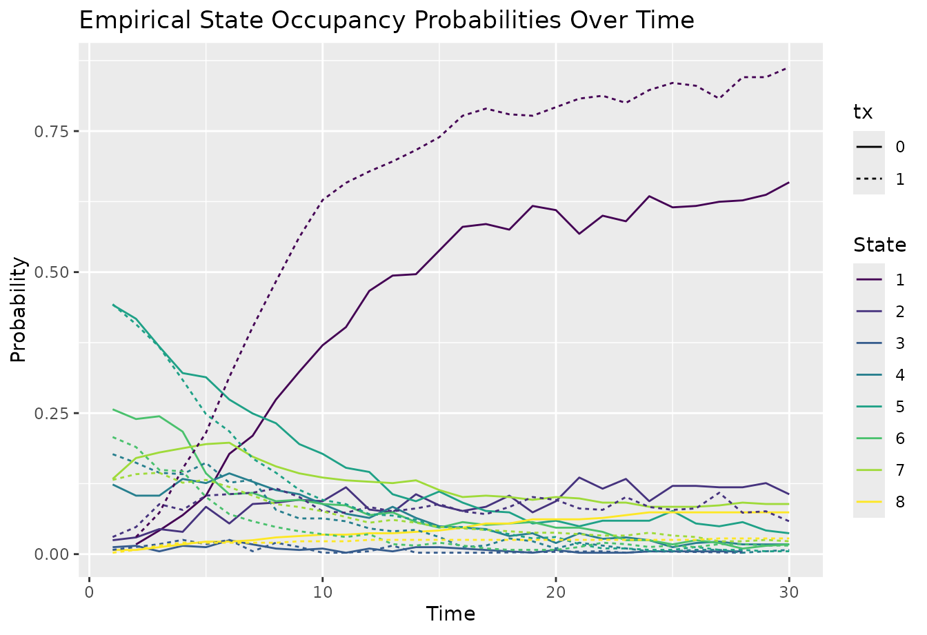

model_data <- prepare_markov_data(
  raw_data,
  absorbing_state = as.integer(ABSORB)
)

dd <- rms::datadist(model_data)
options(datadist = "dd")

fit <- orm_markov(
  y ~ tx + time + yprev,
  data = model_data,
  id_var = "id",
  opt_method = "LM",
  scale = TRUE,
  maxit = 100
)

Choose conditional or unconditional variance

An averaged SOP, such as the probability of being at home on day 14 if every patient had received treatment, depends on two things: the model coefficients and the patients over whom we average. The vcov argument of inferences() decides which of these count as uncertain.

• Conditional variance, vcov = "conditional", accounts for uncertainty in the estimated coefficients but treats the patients’ starting states and covariates as given. It answers: how precisely have we estimated the average for these particular patients?
• Unconditional variance, vcov = "unconditional", additionally accounts for which patients happened to be sampled, and for the fact that the same patients were used to estimate the coefficients. It answers: how precisely have we estimated the average in the population the patients were drawn from?

Both give the same point estimates; only the standard errors and confidence intervals differ. Unconditional intervals are usually wider, most visibly early in follow-up, when SOPs depend strongly on the patients’ starting states.

Averaged SOPs from avg_sops() and comparisons from avg_comparisons() use unconditional variance by default. Patient-level SOPs from sops() support only conditional variance, since there is no average over sampled patients.

Conditional variance

Let \(i = 1,\ldots,n\) index patients, and let \(\beta\) be the vector of all \(p\) model coefficients, with estimate \(\hat\beta\). For patient \(i\), the column vector \(h_i(\beta)\) stacks the predicted probabilities \(S_{it}(l)\) for all requested times \(t\) and states \(l\). Write \(h_i = h_i(\hat\beta)\) for the fitted values and \(\bar h = n^{-1}\sum_{i=1}^n h_i\) for their average, which is what avg_sops() reports.

The matrix \(G_i\) describes how patient \(i\)’s predictions change with the coefficients: it contains the derivatives of \(h_i(\beta)\) with respect to \(\beta^\top\) at \(\hat\beta\), with one row per prediction and one column per coefficient. The average prediction changes according to \(\bar G = n^{-1}\sum_{i=1}^n G_i\). If \(V_\beta\) is the estimated covariance matrix of the coefficients, the conditional covariance matrix of the averaged SOPs is

\[ \bar G V_\beta \bar G^\top. \]

The square roots of its diagonal entries are the standard errors.

By default, \(V_\beta\) is the fit’s patient-cluster robust covariance, which allows for the correlation between a patient’s repeated transitions. There are two fitting options in orm_markov() and vglm_markov() that allow adjustment for small samples:

• type = "HC1" multiplies it by \((m - 1)/(m - p)\), where \(m\) is the number of rows used in fitting (rows with positive weight, for orm_markov()) and \(p\) is the number of coefficients. type = "HC0" applies no such factor, and is used by default.
• cadjust = TRUE multiplies it by \(n/(n - 1)\), where \(n\) is the number of patients. Fits with id_var use this adjustment by default.

Conditional variance, like MVN simulation, also works for weighted and penalized orm_markov() fits whose fitted covariance is valid.

# compute sops
t1 <- Sys.time()
avg_conditional <- avg_sops(
  fit,
  variables = list(tx = c(0, 1)),
  times = seq_len(FOLLOW_UP),
  y_levels = fit$yunique,
  absorb = ABSORB
) |> inferences(
  method = "delta",
  vcov = "conditional",
  conf_type = "auto"
)
t2 <- Sys.time()
t2 - t1

#> Time difference of 1.084971 secs

# compute time in state
time_conditional <- avg_time(
  fit,
  variables = list(tx = c(0, 1)),
  times = seq_len(FOLLOW_UP),
  y_levels = fit$yunique,
  absorb = ABSORB
) |>
  inferences(
    method = "delta",
    vcov = "conditional", 
  )

# compute differences in time in state
comp_conditional <- avg_comparisons(
  fit,
  variables = list(tx = c(0, 1)),
  times = seq_len(FOLLOW_UP),
  y_levels = fit$yunique,
  absorb = ABSORB,
  estimand = "time_in_state",
  comparison = "difference"
) |>
  inferences(
    method = "delta",
    vcov = "conditional", 
    # specify null hypothesis, here no difference on additive scale
    null = 0
  )

p1.sops <- plot_sops(avg_conditional, linetype_var = "tx", facet_var = NULL) +
  labs(title = "Conditional variance")

p1.c <- plot_comparisons(comp_conditional) +
  labs(title = "Conditional variance")

Unconditional variance

The unconditional calculation adds a second source of variation: had a different set of patients enrolled, both the average of their predictions and the fitted coefficients would have changed, and these two changes are related. Each patient’s contribution to both is captured in one vector,

\[ \phi_i = h_i - \bar h + \bar G A^{-1}s_i. \]

The first part, \(h_i - \bar h\), is how far patient \(i\)’s predictions lie from the average. The second part is the patient’s influence on the coefficients, translated into its effect on the average prediction through \(\bar G\). In it,

• \(s_i = \sum_{r \in \mathcal{I}_i}\psi_r\) is the patient’s score: the sum, over the patient’s fitting rows \(\mathcal{I}_i\), of the derivatives \(\psi_r = \partial\ell_r/\partial\beta\) of each row’s log-likelihood \(\ell_r\), evaluated at \(\hat\beta\);
• \(A^{-1} = nB\), where \(B\) is the inverse of the fit’s total information matrix, before any type or cadjust correction. With the default observed information, \(A\) is the negative derivative of the average patient score; a fit that uses a different (working) information matrix uses that matrix instead.

Thus \(A^{-1}s_i\) approximates how much patient \(i\) moves the estimated coefficients. The unconditional covariance matrix is the sample covariance of the \(\phi_i\) divided by \(n\):

\[ V_{\mathrm{unconditional}} = \frac{1}{n(n-1)} \sum_{i=1}^n (\phi_i - \bar\phi)(\phi_i - \bar\phi)^\top, \qquad \bar\phi = n^{-1}\sum_{i=1}^n \phi_i. \]

In R terms, this is stats::cov(phi) / n, where stats::cov() uses the usual divisor \(n - 1\). Because the two parts of \(\phi_i\) are combined before taking the covariance, their correlation in the observed sample is retained. The fitting options type and cadjust do not change this estimate.

avg_unconditional <- avg_sops(
  fit,
  variables = list(tx = c(0, 1)),
  times = seq_len(FOLLOW_UP),
  y_levels = fit$yunique,
  absorb = ABSORB
) |> inferences(
  method = "delta",
  vcov = "unconditional",
  conf_type = "wald"
)

# compute time in state
time_unconditional <- avg_time(
  fit,
  variables = list(tx = c(0, 1)),
  times = seq_len(FOLLOW_UP),
  y_levels = fit$yunique,
  absorb = ABSORB
) |>
  inferences(
    method = "delta",
    vcov = "unconditional", 
  )


comp_unconditional <- avg_comparisons(
  fit,
  variables = list(tx = c(0, 1)),
  times = seq_len(FOLLOW_UP),
  y_levels = fit$yunique,
  absorb = ABSORB,
  estimand = "time_in_state",
  comparison = "difference"
) |>
  inferences(
    method = "delta",
    vcov = "unconditional",
    null = 0
  )

p2.sops <- plot_sops(avg_unconditional, linetype_var = "tx", facet_var = NULL) +
  labs(title = "Unconditional variance")

p2.c <- plot_comparisons(comp_unconditional) +
  labs(title = "Unconditional variance")

The plots below compare the two choices, first for the SOPs and then for the differences in expected time in each state (treated minus control). The point estimates are identical; the intervals differ.

p1.sops + p2.sops + plot_layout(guides = "collect")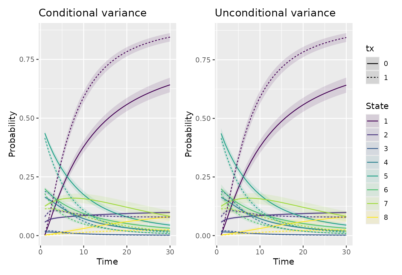

p1.c + p2.c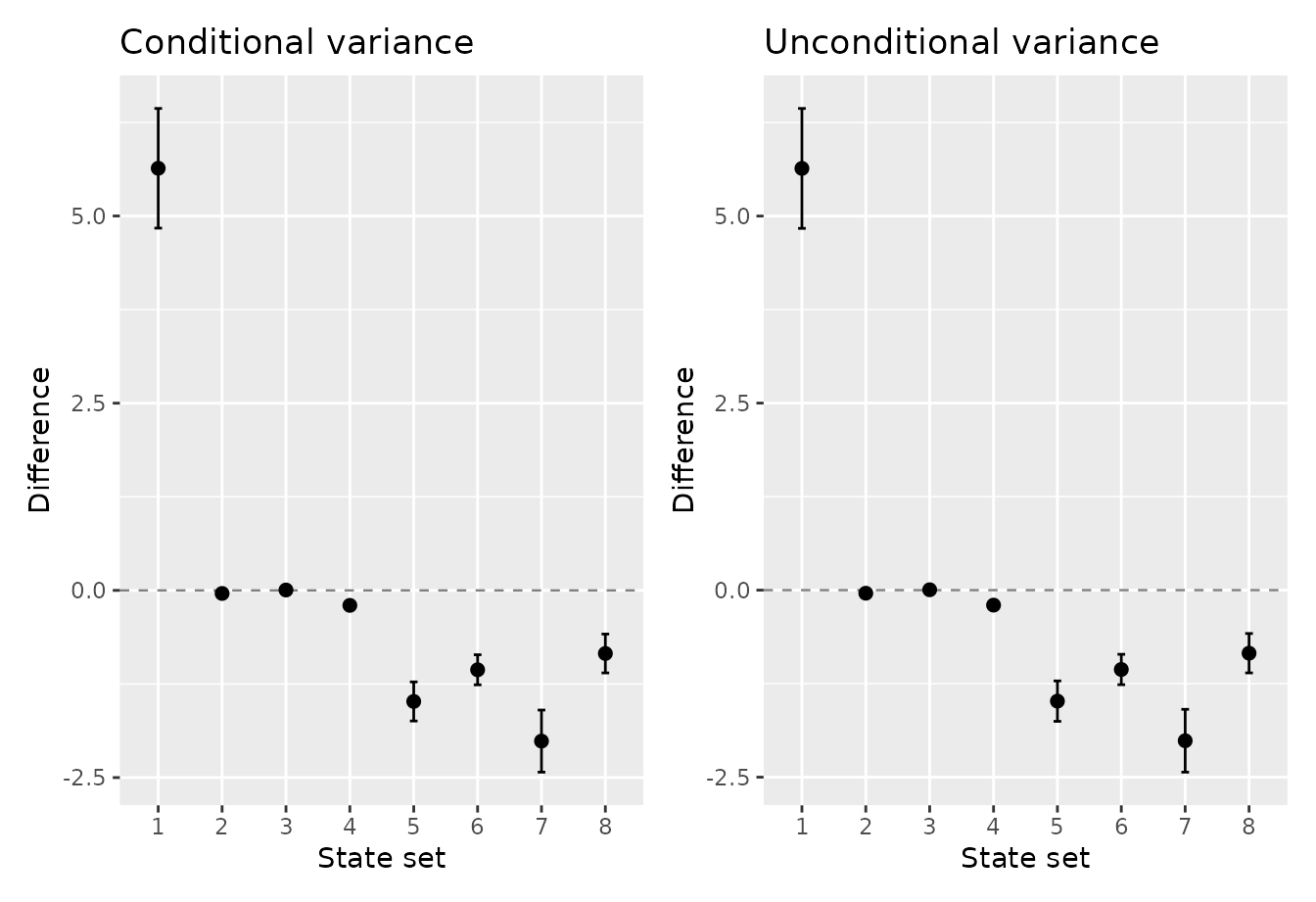

We can also plot the expect time in each state by arm using Grotta bars:

plot_time(time_conditional, show_labels = FALSE)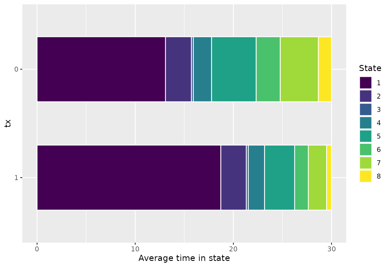

If we want to show uncertainty, we can plot the expected time differently as well:

plot_time(time_conditional, show_labels = FALSE, type = "pointrange")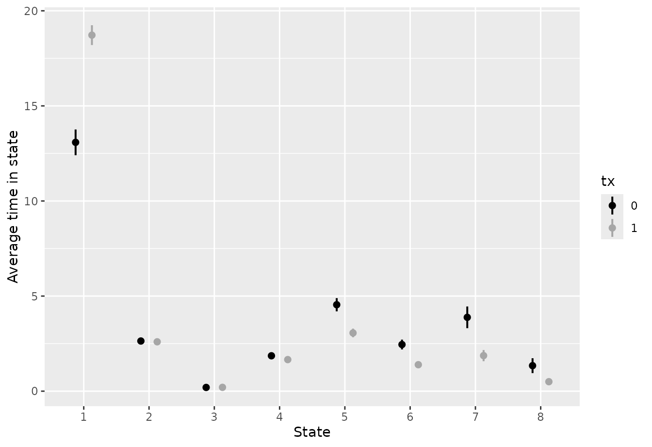

Requirements for unconditional variance

Unconditional variance needs each patient’s scores, so it is available only when

• the model was fitted with orm_markov() or vglm_markov(), which store the patient information needed; models fitted directly with rms::orm() or VGAM::vglm() cannot be used for analytical intervals at all;
• the average is taken over the patients stored with the model, not over user-supplied newdata; and
• the orm_markov() fit is neither weighted nor penalized.

If a requirement is not met, inferences() stops with an error rather than silently switching to conditional variance. With newdata, for example, request vcov = "conditional" explicitly.

Which patients are included in the average?

Without newdata, predictions start from each fitted patient’s row at the first follow-up time, first_followup_time: that row supplies the patient’s starting state (yprev) and covariates. The model stores these rows before dropping rows with missing outcomes. Therefore:

• each patient must have exactly one row at that time, with ID, predictors, time, and yprev all observed;
• the outcome on that row may be missing, provided the patient contributes at least one other transition to the fit;
• a later row cannot stand in for missing starting information.

For numeric time, first_followup_time defaults to 1, which must be the earliest scheduled time. If you set another value, it must still be the earliest. For factor or character time, you must set it explicitly; see vignette("factor-time-orm-sops").

Neither variance corrects bias caused by missing observations whose missingness depends on unobserved outcomes.

Why patient IDs matter

Each patient contributes many transitions to the model, and these are not independent. Treating them as independent would typically make standard errors too small. mostr therefore groups the fitting rows by patient, identifying patients as follows:

1. If you pass cluster to inferences(), its entries identify the patient for each fitting row, in the order of the fitting data.
2. Otherwise, mostr uses the id_var column given to orm_markov() or vglm_markov().
3. Without patient IDs, patient-cluster robust variance cannot be calculated.

For conditional variance, you can instead supply your own coefficient covariance matrix through vcov. It must cover all model coefficients, with matching names. Supplying a matrix always selects conditional variance, because a matrix alone does not carry the patient-level scores that unconditional variance needs.

Grouping by patient corrects the standard errors for within-patient correlation. It does not correct for a transition model that describes the data poorly, nor for bias from missing observations.

Logit and Wald intervals

conf_type controls how confidence limits are formed from the estimate and its standard error.

• conf_type = "auto", the default, forms intervals for probabilities on the logit scale and transforms the limits back. This keeps them between 0 and 1.
• conf_type = "wald" uses the estimate plus or minus a normal quantile times the standard error. Its limits can fall below 0 or above 1.

Differences between arms can be negative, so analytical intervals for differences always use the Wald form; conf_type = "auto" selects it automatically.

If an estimated probability is exactly 0 or 1, its logit is undefined and the logit-scale limits are returned as NA with a warning, even when the standard error is 0. Such values can arise from rounding and do not necessarily mean that the outcome is certain. This applies to absorbing states too: patients who enter one stay there, but the probability of entering it is still estimated.

Each interval covers one estimate at the stated confidence level. The level does not apply jointly to all intervals.

The example below compares the average probability of being outside hospital (states 1 and 2 combined) between arms, as treated minus control.

sop_difference <- avg_comparisons(
  fit,
  variables = list(tx = c(0, 1)),
  estimand = "sop",
  state_sets = c("1", "2"),
  comparison = "difference",
  times = seq_len(FOLLOW_UP),
  y_levels = fit$yunique,
  absorb = ABSORB
) |>
  inferences(
    method = "delta",
    vcov = "conditional",
    conf_type = "auto"
  )

head(sop_difference)

Show output

#>   estimand time state_set term reference_level comparison_level contrast
#> 1      sop    1       1+2   tx               0                1    1 - 0
#> 2      sop    2       1+2   tx               0                1    1 - 0
#> 3      sop    3       1+2   tx               0                1    1 - 0
#> 4      sop    4       1+2   tx               0                1    1 - 0
#> 5      sop    5       1+2   tx               0                1    1 - 0
#> 6      sop    6       1+2   tx               0                1    1 - 0
#>   comparison   estimate   std.error statistic      p.value  s.value   conf.low
#> 1 difference 0.02442457 0.001881880  12.97881 1.613621e-38 125.5430 0.02073616
#> 2 difference 0.06010226 0.004543741  13.22748 6.089186e-40 130.2709 0.05119669
#> 3 difference 0.09537444 0.007102533  13.42823 4.131719e-41 134.1523 0.08145373
#> 4 difference 0.12629464 0.009283731  13.60387 3.798044e-42 137.5957 0.10809887
#> 5 difference 0.15188351 0.011054653  13.73933 5.902080e-43 140.2817 0.13021678
#> 6 difference 0.17231621 0.012457397  13.83244 1.624134e-43 142.1432 0.14790016
#>    conf.high
#> 1 0.02811299
#> 2 0.06900782
#> 3 0.10929515
#> 4 0.14449042
#> 5 0.17355023
#> 6 0.19673226

The standard error of a difference accounts for both arms’ predictions coming from the same fitted model and the same patients; the two arms are not treated as independent.

estimand = "time_in_state" compares the expected time spent in a state instead, as in the plots above. For visits recorded as a factor, supply the elapsed time of each visit; vignette("factor-time-orm-sops") shows how, and how to include the observed baseline state.

Extract variances and covariances

The output of inferences() already contains standard errors and confidence limits. To learn how the uncertainty in different estimates is related, for example to test a combination of estimates yourself, use vcov(). It returns the covariance matrix of the estimates: its diagonal entries are variances, and the off-diagonal entries are covariances between pairs of estimates. The matrix reflects the conditional or unconditional choice made in inferences().

The example requests the first six estimates only. The square roots of the diagonal are their standard errors, matching the std.error column.

rows <- seq_len(min(6L, nrow(avg_conditional)))

conditional_covariance <- stats::vcov(avg_conditional, rows = rows)
unconditional_covariance <- stats::vcov(avg_unconditional, rows = rows)

sqrt(diag(conditional_covariance))

#>     1\r1\r0     2\r1\r0     3\r1\r0     4\r1\r0     5\r1\r0     6\r1\r0 
#> 0.000186052 0.002331517 0.004498137 0.006499989 0.008220933 0.009639445

sqrt(diag(unconditional_covariance))

#>      1\r1\r0      2\r1\r0      3\r1\r0      4\r1\r0      5\r1\r0      6\r1\r0 
#> 0.0001975683 0.0037044533 0.0061500033 0.0080427528 0.0096023821 0.0108847730

Without rows, vcov() returns a covariance for every pair of estimates. This can use a lot of memory, because doubling the number of estimates quadruples the number of entries, so request only the rows you need. The option mostr.delta_max_bytes, 256 MiB by default, caps the largest memory allocations made by analytical inference and by vcov().

If you want to see the derivatives \(\bar G\) themselves, the internal function below returns them for the selected estimates: one row per estimate and one column per coefficient. They enter both variances, but they do not include the patient-sampling part of the unconditional variance.

coefficient_derivatives <- mostr:::get_jacobian(avg_conditional, rows = rows)
coefficient_derivatives

Show output

#>                 y>=2        y>=3          y>=4         y>=5          y>=6
#> 1\r1\r0 -0.001132096  0.00000000  0.0000000000  0.000000000  0.0000000000
#> 2\r1\r0 -0.007897314 -0.03831245 -0.0005617418 -0.000552515 -0.0000205348
#> 3\r1\r0 -0.014889904 -0.05684628 -0.0120334389 -0.023947529 -0.0012861407
#> 4\r1\r0 -0.021418085 -0.06775362 -0.0215985495 -0.054444192 -0.0059654399
#> 5\r1\r0 -0.027381303 -0.07428878 -0.0290197864 -0.084149822 -0.0137423083
#> 6\r1\r0 -0.032780378 -0.07805951 -0.0346634556 -0.110222302 -0.0235881328
#>                  y>=7          y>=8 tx         time      yprev=2       yprev=3
#> 1\r1\r0  0.000000e+00  0.000000e+00  0 -0.001132096  0.000000000  0.0000000000
#> 2\r1\r0 -1.562830e-07 -8.915904e-11  0 -0.055244435 -0.006472823 -0.0002455501
#> 3\r1\r0 -1.164646e-05 -7.617800e-09  0 -0.178647307 -0.007804784 -0.0035469850
#> 4\r1\r0 -1.500138e-04 -1.566666e-07  0 -0.362575448 -0.008386908 -0.0061036095
#> 5\r1\r0 -6.627916e-04 -1.256310e-06  0 -0.595549939 -0.008782520 -0.0079874248
#> 6\r1\r0 -1.742042e-03 -5.401704e-06  0 -0.866066782 -0.009086313 -0.0093624370
#>               yprev=4       yprev=5       yprev=6       yprev=7
#> 1\r1\r0 -0.0009821635 -0.0001486524 -1.275389e-06 -4.301474e-09
#> 2\r1\r0 -0.0314564092 -0.0089479204 -9.156997e-05 -3.610841e-07
#> 3\r1\r0 -0.0581727996 -0.0325167493 -9.977764e-04 -7.038963e-06
#> 4\r1\r0 -0.0803894811 -0.0604663709 -3.729421e-03 -5.125895e-05
#> 5\r1\r0 -0.0981477259 -0.0877595745 -8.257507e-03 -1.929785e-04
#> 6\r1\r0 -0.1119021577 -0.1124334843 -1.419358e-02 -4.888766e-04

Supported models and comparisons

Analytical confidence intervals are available for:

• first-order Markov models, where the next state depends only on the previous state and the covariates;
• full proportional-odds models with a reverse cumulative-logit link;
• frequentist models fitted with orm_markov() or vglm_markov() (including the robcov_vglm object that vglm_markov() returns);
• patient-level SOPs from sops() with conditional variance, and averaged SOPs from avg_sops() with conditional or unconditional variance;
• differences with estimand = "sop" or estimand = "time_in_state"; and
• numeric or factor visit times.

For other models, such as partial proportional-odds or second-order models, or for estimand = "time_benefit", use simulation or the bootstrap; see vignette("mvn-vs-bootstrap-orm-sops").