MVN Simulation Versus Bootstrap for orm_markov() SOPs

Analytical confidence intervals (vignette("analytical-confidence-intervals")) are not available for every model or summary. Two general alternatives work with frequentist models fitted by orm_markov() or vglm_markov():

1. Multivariate-normal (MVN) simulation, method = "mvn", draws many coefficient vectors from a multivariate normal distribution centered on the estimates, with the model’s covariance matrix. For each draw it recomputes the state occupancy probabilities (SOPs) over the same patients. The spread of the results reflects uncertainty in the coefficients only, with the patients’ starting states and covariates treated as given, like the conditional variance of the analytical method.
2. Patient bootstrap, method = "bootstrap", resamples patients with replacement, refits the model to each resample, and recomputes the averaged SOPs over the resampled patients. Its spread reflects both uncertainty in the coefficients and which patients happened to be sampled, like the unconditional variance of the analytical method.

MVN simulation is much faster, because it never refits the model. The bootstrap relies less on the normal approximation to the coefficients and also reflects variation in the patients averaged over, but refitting can take a long time for large models.

This article applies both methods to the same fitted model and compares the results. It uses only 50 draws so that it runs quickly; a real analysis needs many more, typically 1,000 or more, for stable interval limits.

Simulate data and fit the model

We simulate 200 patients over 10 days with sim_markov("actt2"), which uses the eight-state NIAID scale described in vignette("full-po-sops"), and fit a proportional-odds transition model.

library(mostr)
library(ggplot2)
library(rms)

N_PATIENTS <- 200
FOLLOW_UP <- 10
N_DRAWS <- 50
SEED <- 20260602
STATE_LEVELS <- as.character(1:8)
ABSORB <- "8"

raw_data <- sim_markov(
  "actt2",
  n_patients = N_PATIENTS,
  follow_up_time = FOLLOW_UP,
  treatment_effect = log(0.8),
  seed = SEED
)

model_data <- prepare_markov_data(raw_data, absorbing_state = as.integer(ABSORB))

dd <- rms::datadist(model_data)
options(datadist = "dd")

fit_orm <- orm_markov(
  y ~ tx + rms::rcs(time, 4) + yprev,
  data = model_data,
  id_var = "id",
  opt_method = "LM",
  scale = TRUE,
  maxit = 100
)

Both methods rely on what orm_markov() stores with the fit. With id_var = "id", it computes a covariance matrix that allows for correlation between each patient’s transitions, which MVN simulation draws from. It also keeps the full longitudinal data, which the bootstrap resamples and refits, and each patient’s starting row, over which avg_sops() averages.

Estimate SOPs

The point estimates are computed once, and both methods start from the same object.

avg <- avg_sops(
  fit_orm,
  variables = list(tx = c(0, 1)),
  times = seq_len(FOLLOW_UP),
  y_levels = fit_orm$yunique,
  absorb = ABSORB
)

Run both methods

workers sets the number of parallel processes; more than one speeds up the bootstrap considerably. return_draws = TRUE keeps the individual draws, which get_draws() extracts for further analysis. Setting the seed makes the draws reproducible.

set.seed(SEED)
sop_mvn <- inferences(
  avg,
  method = "mvn",
  n_draws = N_DRAWS,
  workers = 1,
  return_draws = TRUE
)

set.seed(SEED)
sop_boot <- inferences(
  avg,
  method = "bootstrap",
  n_draws = N_DRAWS,
  workers = 1,
  return_draws = TRUE
)

Compare the results

comparison <- rbind(
  data.frame(method = "MVN simulation", as.data.frame(sop_mvn)),
  data.frame(method = "Patient bootstrap", as.data.frame(sop_boot))
)

plot_sops(
  comparison,
  geom = "line",
  facet_var = c("method"),
  linetype_var = "tx"
) +
  labs(
    x = "Day",
    y = "State occupancy probability"
  )

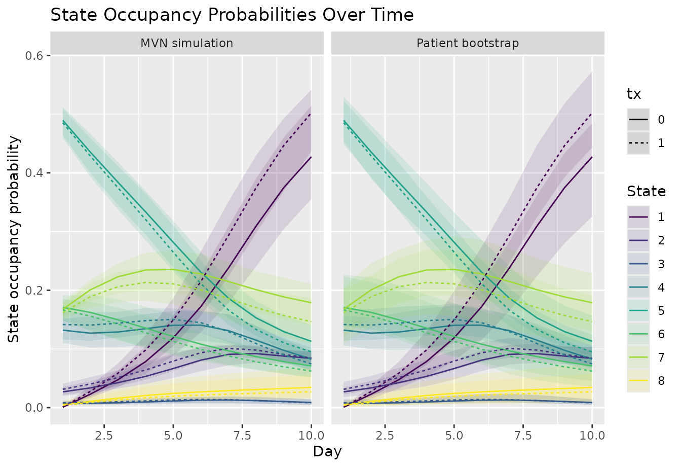
The point estimates are identical, because both come from the same fitted model. The intervals differ because the two methods answer different questions. MVN simulation measures how precisely the average is known for these 200 patients. The bootstrap measures how precisely it is known for the population they were sampled from, so it also captures variation in the patients’ starting states. The difference is largest in the first days, when the SOPs depend most strongly on where patients started. Magirr et al. (2025) discuss this distinction for covariate-adjusted treatment effects in randomized trials.

References

Magirr D, Wang C, Przybylski A, Baillie M. Estimating the variance of covariate-adjusted estimators of average treatment effects in clinical trials with binary endpoints. Pharmaceutical Statistics. 2025;24(4):e70021. doi:10.1002/pst.70021