Many Outcome Levels with a Previous-State Spline • mostr

Some outcomes have many ordered levels, such as a quality-of-life score from 1 to 30. Treating the previous state as a factor then adds one coefficient per level, 29 in this case, and the rarer levels are poorly estimated. Instead, the previous state can enter the model as a number, with a restricted cubic spline allowing its effect to be non-linear. This uses a handful of coefficients however many levels there are.

This article fits such a model, checks it against the data, and compares arms using three summaries: state occupancy probabilities (SOPs), expected time in each state, and time benefit.

Simulate an outcome with 30 levels

We simulate 220 patients over 14 days on a 30-level scale where higher is worse and no state is absorbing. sim_markov() with preset = NULL generates each day’s state from an ordinal model whose linear predictor is supplied in lp_function: it increases linearly with the previous state, decreases slightly over time, and is shifted by treatment_effect = -0.25 for treated patients. The 29 cut-points are spread so that, with a linear predictor of zero, the 30 states are equally likely.

library(mostr)
library(ggplot2)
library(rms)

N_PATIENTS <- 220
FOLLOW_UP <- 14
N_QOL <- 30
STATE_LEVELS <- as.character(seq_len(N_QOL))
ABSORB <- NULL
SEED <- 20260530

set.seed(SEED)
baseline <- data.frame(
  id = seq_len(N_PATIENTS),
  yprev = sample(12:28, N_PATIENTS, replace = TRUE),
  tx = rbinom(N_PATIENTS, 1, 0.5)
)
raw_data <- sim_markov(
  NULL,
  baseline_data = baseline,
  follow_up_time = FOLLOW_UP,
  intercepts = qlogis(seq_len(N_QOL - 1L) / N_QOL),
  absorbing_states = integer(),
  covariate_names = "tx",
  treatment_effect = -0.25,
  lp_function = function(yprev, t, tx, treatment_effect, extra_params) {
    0.08 * (as.numeric(as.character(yprev)) - 15) - 0.03 * t +
      treatment_effect * tx
  },
  seed = SEED
)

plot_sops(raw_data, geom = "bar")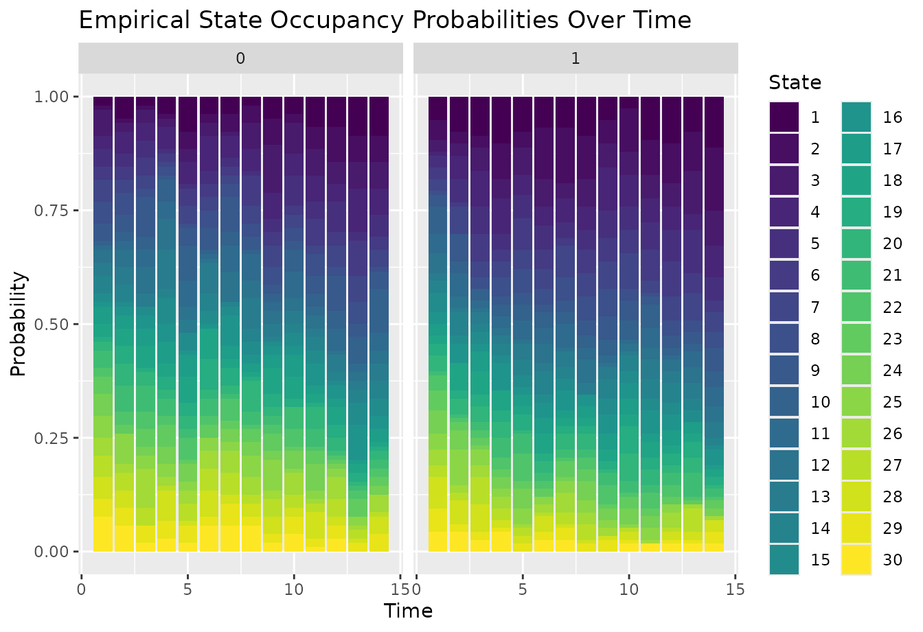

Fit a spline in the previous state

prepare_markov_data(..., factor_previous = FALSE) keeps yprev numeric so that it can enter the model through rcs(yprev, 5), a restricted cubic spline with five knots. Because no state is absorbing, absorbing_state = NULL.

model_data <- prepare_markov_data(
  raw_data,
  absorbing_state = NULL,
  factor_previous = FALSE
)

dd <- rms::datadist(model_data)
options(datadist = "dd")

fit_many <- orm_markov(
  y ~ rms::rcs(time, 4) + tx + rms::rcs(yprev, 5),
  data = model_data,
  id_var = "id",
  opt_method = "LM",
  scale = TRUE,
  penalty = 0,
  maxit = 100
)

fit_many

Show output

#> Logistic (Proportional Odds) Ordinal Regression Model
#> 
#> rms::orm(formula = y ~ rms::rcs(time, 4) + tx + rms::rcs(yprev, 
#>     5), data = model_data, opt_method = "LM", scale = TRUE, penalty = 0, 
#>     maxit = 100, x = TRUE, y = TRUE)
#> 
#>                          Model Likelihood               Discrimination    Rank Discrim.    
#>                                Ratio Test                      Indexes          Indexes    
#> Obs            3080    LR chi2     599.70    R2                  0.177    rho     0.421    
#> ESS          3075.4    d.f.             8    R2(8,3080)          0.175    Dxy     0.299    
#> Distinct Y       30    Pr(> chi2) <0.0001    R2(8,3075.4)        0.175                     
#> Cluster on  cluster                          |Pr(Y>=median)-0.5| 0.163                     
#> Clusters        220                                                                        
#> Median Y         12                                                                        
#> max |deriv|  0.0007                                                                        
#> 
#>          Coef    S.E.   Wald Z Pr(>|Z|)
#> time     -0.0585 0.0425 -1.38  0.1684  
#> time'     0.0918 0.1309  0.70  0.4831  
#> time''   -0.2909 0.3269 -0.89  0.3735  
#> tx       -0.3526 0.0600 -5.88  <0.0001 
#> yprev     0.1083 0.0439  2.46  0.0137  
#> yprev'   -1.7217 1.4937 -1.15  0.2491  
#> yprev''   2.3175 1.9262  1.20  0.2289  
#> yprev''' -0.9665 0.6389 -1.51  0.1304

Check the model against the data

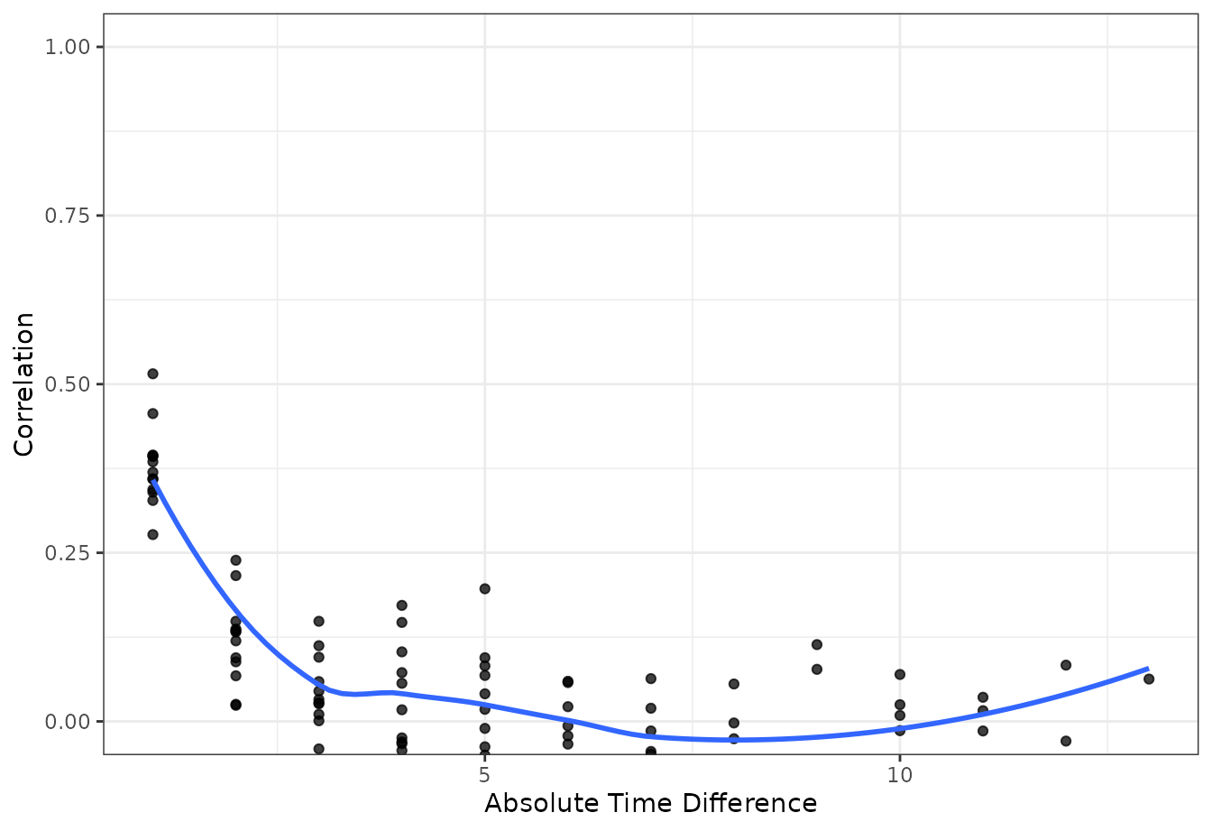
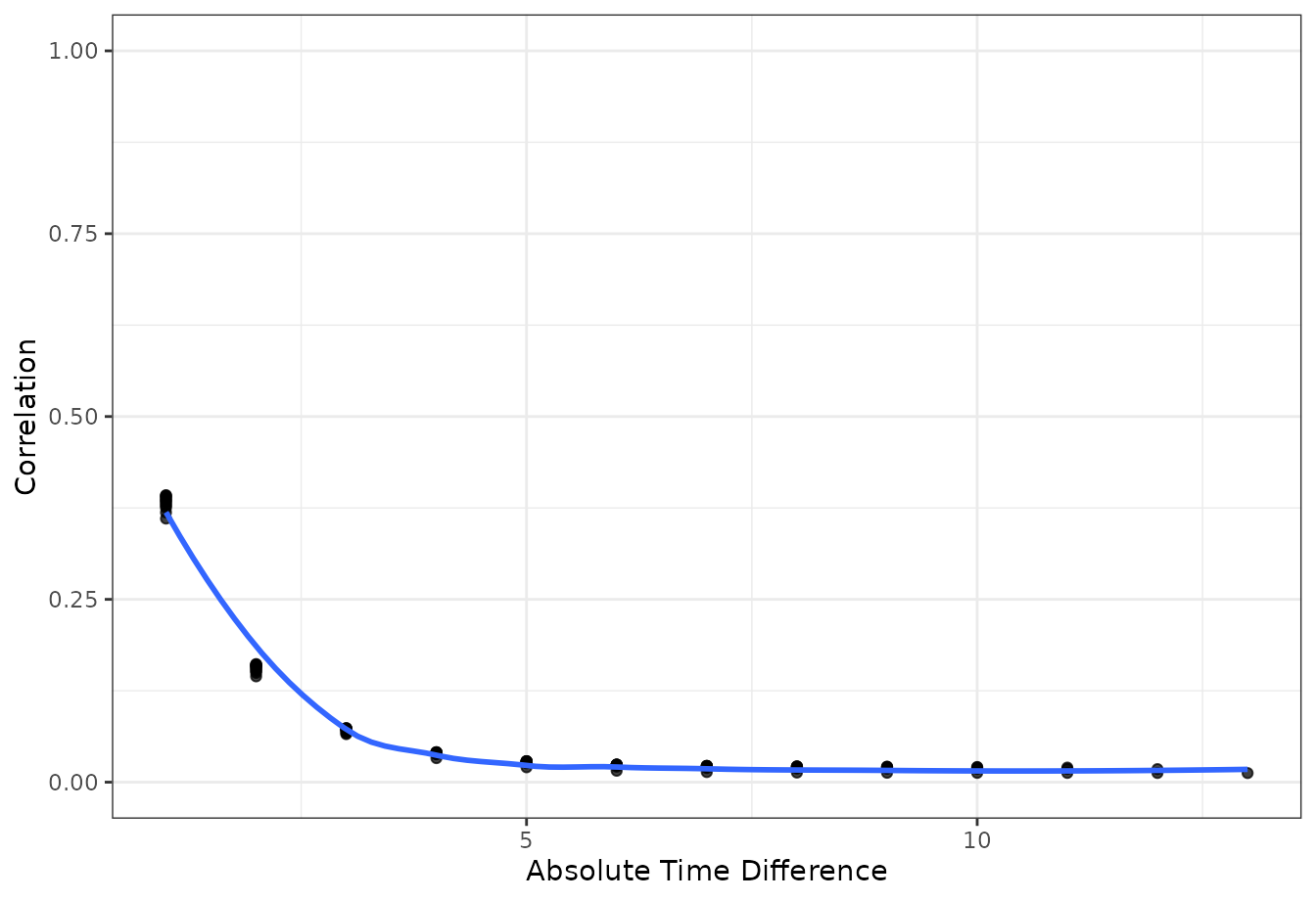
As in vignette("full-po-sops"), we compare the correlations between days in the observed data with those implied by the model, first as a matrix of all pairs of days and then as a variogram against the gap between days. Without an absorbing state, absorb = NULL. Some observed correlations are slightly negative, so both correlation plots use fill_limits = c(-1, 1); a shared scale makes their colors comparable.

ec <- plot_correlation(
  fill_limits = c(-1, 1),
  show_values = FALSE,
  raw_data,
  id_var = "id",
  time_var = "time",
  y_var = "y"
)

mc <- plot_correlation(
  fill_limits = c(-1, 1),
  show_values = FALSE,
  fit_many,
  id_var = "id",
  time_var = "time",
  y_var = "y",
  times = seq_len(FOLLOW_UP),
  y_levels = fit_many$yunique,
  absorb = ABSORB
)

ec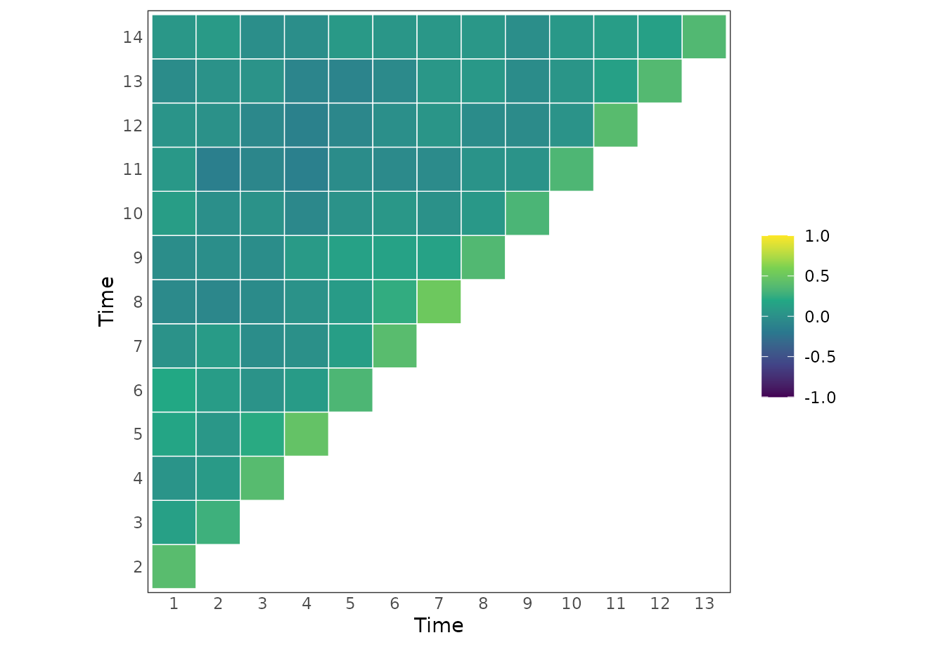

mc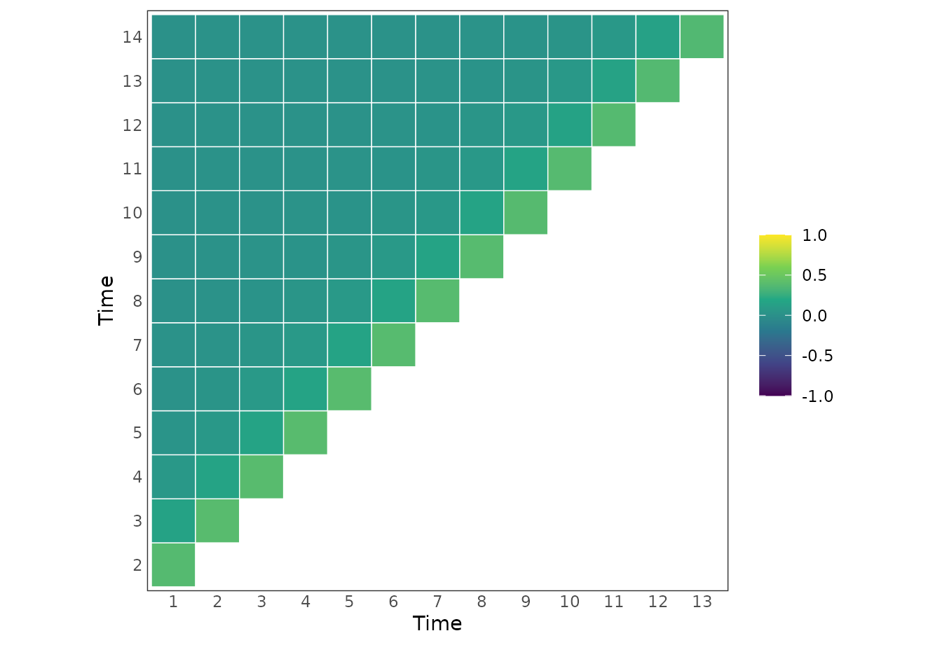

plot_variogram(
  raw_data,
  id_var = "id",
  time_var = "time",
  y_var = "y"
)

plot_variogram(
  fit_many,
  id_var = "id",
  time_var = "time",
  y_var = "y",
  times = seq_len(FOLLOW_UP),
  y_levels = fit_many$yunique,
  absorb = ABSORB
)

Estimate state occupancy probabilities

p_var = "yprev" names the previous-state column. It is the default, shown here to make clear that mostr substitutes each possible previous state into this numeric column, and hence into the spline, when chaining predictions.

sop_many <- avg_sops(
  fit_many,
  variables = list(tx = c(0, 1)),
  times = seq_len(FOLLOW_UP),
  y_levels = fit_many$yunique,
  p_var = "yprev"
) |>
  inferences(method = "delta", vcov = "unconditional")

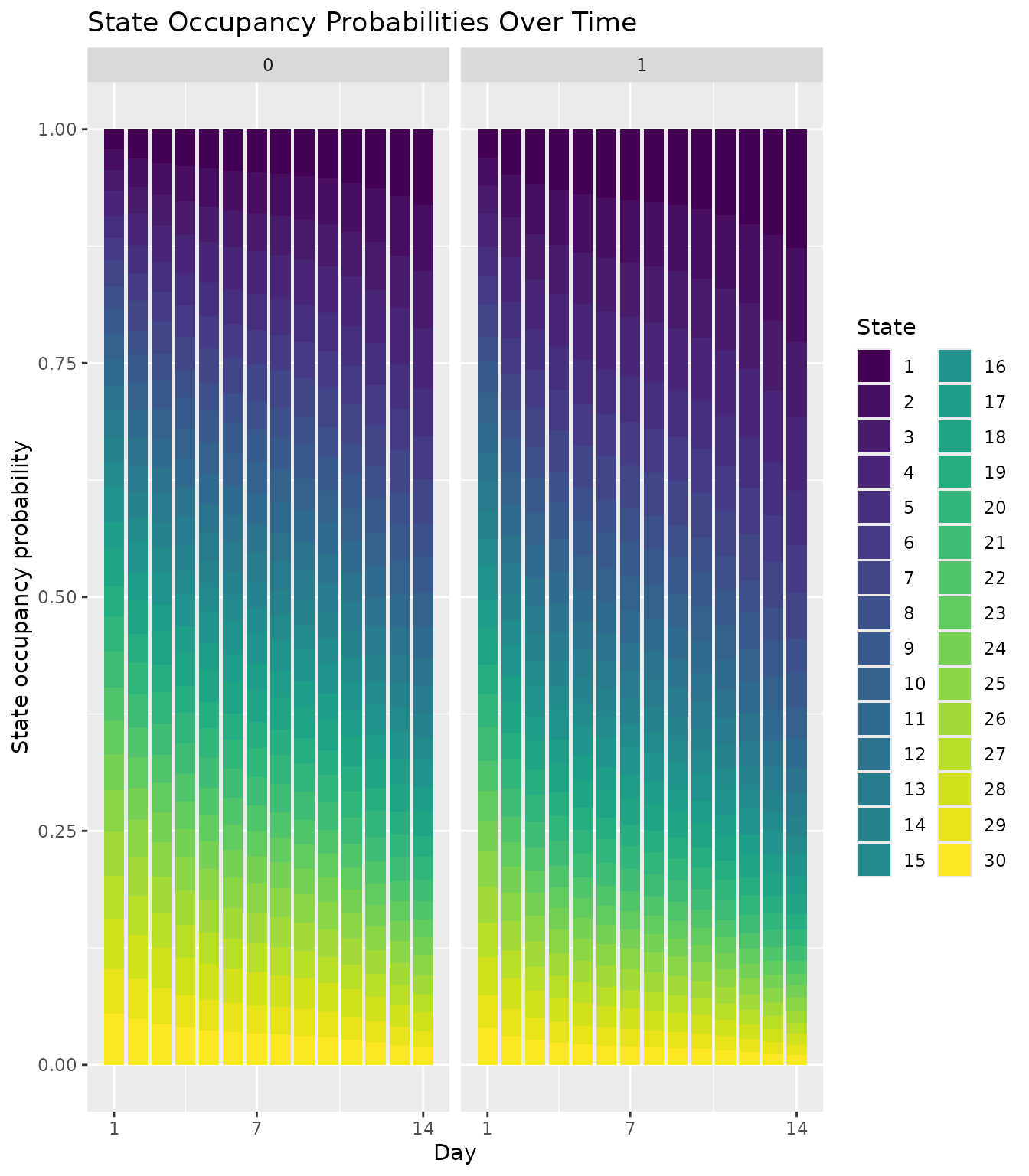
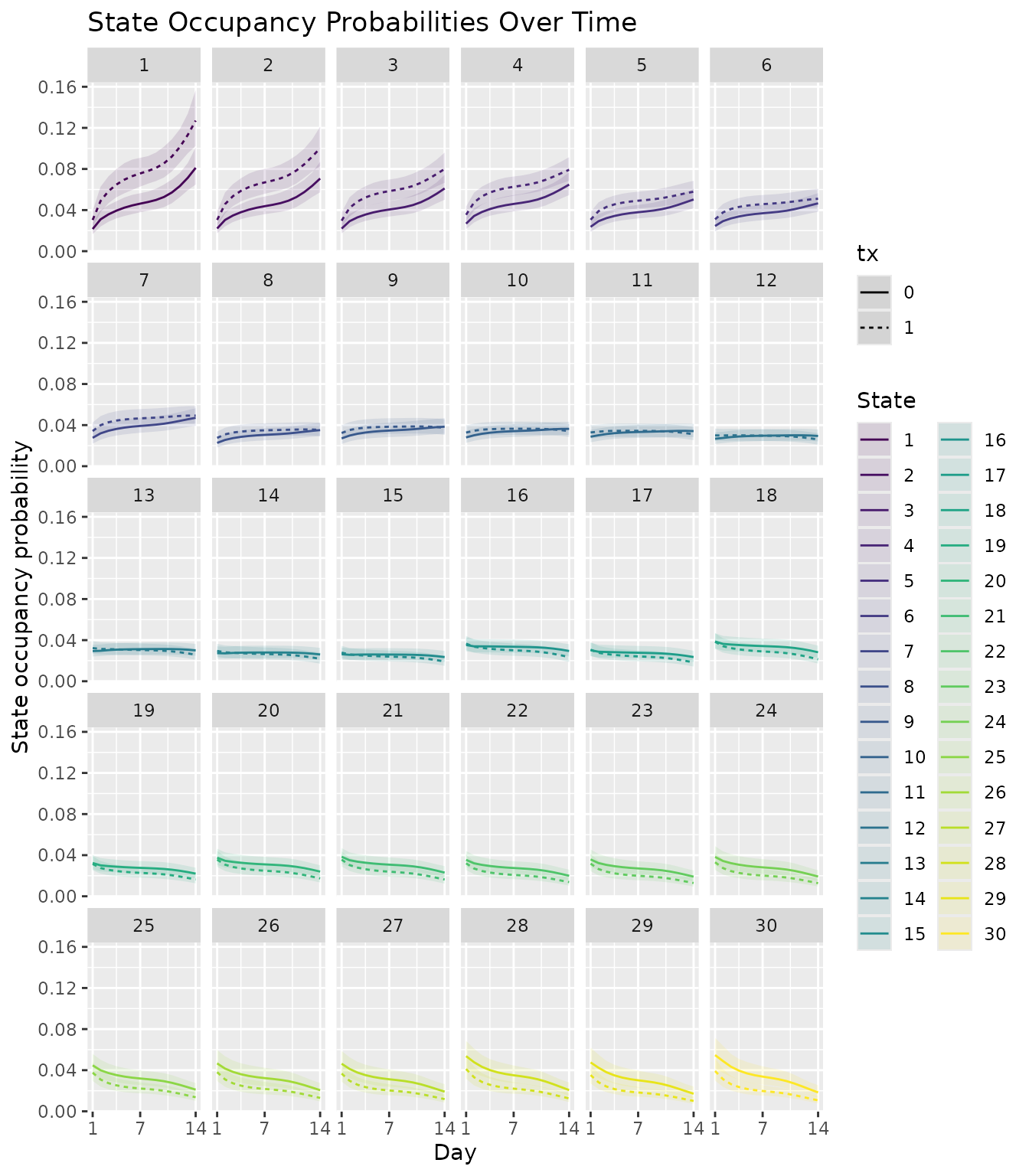
With 30 states, two views help. Stacked bars show the whole distribution on each day, one panel per arm. Line plots, one panel per state, show how each state’s probability changes over time in each arm.

plot_sops(
  sop_many,
  geom = "bar",
  facet_var = "tx"
) +
  scale_x_continuous(breaks = c(1, 7, 14)) +
  labs(
    x = "Day",
    y = "State occupancy probability"
  )

plot_sops(
  sop_many,
  geom = "line",
  facet_var = "state",
  linetype_var = "tx"
) +
  scale_x_continuous(breaks = c(1, 7, 14)) +
  labs(
    x = "Day",
    y = "State occupancy probability"
  )

Compare the arms

Differences in state occupancy probabilities

estimand = "sop" gives, for each state and day, the SOP under treatment minus the SOP under control.

sop_diff <- avg_comparisons(
  fit_many,
  times = seq_len(FOLLOW_UP),
  variables = list(tx = c(0, 1)),
  estimand = "sop"
) |>
  inferences(
    method = "delta",
    vcov = "unconditional"
  )

plot_comparisons(sop_diff, facet_var = "state_set")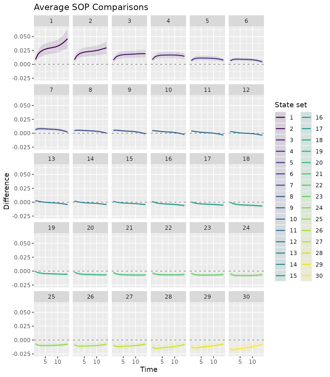

Differences in time in state

estimand = "time_in_state" sums the daily SOPs, giving the expected number of days spent in each state over the 14 days. With many levels, grouping states into bands is often easier to interpret. For example, state_sets = list(good = 1:10, average = 11:20, bad = 21:30) would compare time spent in three bands; here we keep all 30 states.

tis_many <- avg_comparisons(
  fit_many,
  times = seq_len(FOLLOW_UP),
  variables = list(tx = c(0, 1)),
  estimand = "time_in_state"
) |>
  inferences(
    method = "delta",
    vcov = "unconditional"
  )

plot_comparisons(tis_many)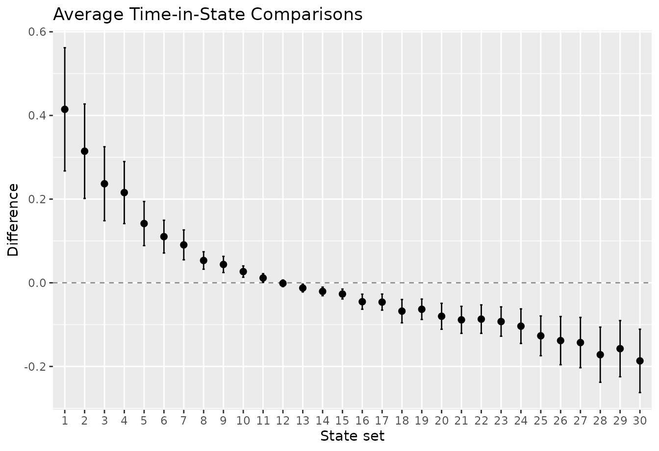

Time benefit

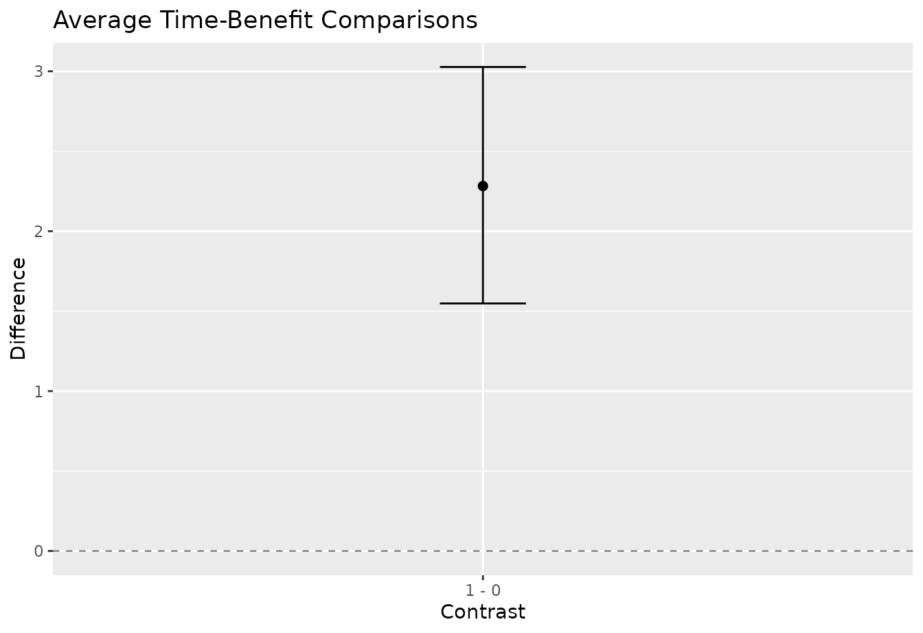
Time benefit summarizes all states in a single number. On each day, imagine drawing one state from each arm’s predicted distribution for the same patient. The daily benefit is the probability that the treated state is better (lower) minus the probability that it is worse. Summing over days gives the expected number of days benefit: the net number of days on which treatment leaves the patient better off. Results are averaged over patients.

Analytical intervals are not yet available for time benefit, so we use simulation from the coefficients’ multivariate normal distribution. Only 50 draws are used here to keep the example fast; use more, such as 1,000, in a real analysis.

tb_many <- avg_comparisons(
  fit_many,
  times = seq_len(FOLLOW_UP),
  variables = list(tx = c(0, 1)),
  estimand = "time_benefit"
) |>
  inferences(
    method = "mvn",
    n_draws = 50
  )

plot_comparisons(tb_many)