Fractional Weighted Bootstrap for SOPs

The ordinary patient bootstrap (vignette("mvn-vs-bootstrap-orm-sops")) draws patients with replacement, so each resample leaves out about a third of the patients and counts others several times. In small samples or subgroups, a resample can then lack patients in a rare state, and the model cannot be refitted, or a subgroup can be missing altogether.

The fractional weighted bootstrap (FWB) avoids this. Instead of resampling, it keeps every patient in every replicate and gives each patient a random positive weight, drawn from an exponential distribution and scaled to have mean 1. For each replicate it

1. refits the transition model, applying each patient’s weight to all of that patient’s rows; and
2. averages the patient-level state occupancy probabilities (SOPs) using the same weights.

Like the ordinary bootstrap, the FWB reflects both uncertainty in the model coefficients and which patients happened to be sampled.

This article uses the FWB to estimate SOPs within subgroups defined by the patients’ starting state, and to compare time benefit between arms in these subgroups.

Fit the model

We simulate 160 patients over 10 days with sim_markov("actt2"), which uses the eight-state NIAID scale described in vignette("full-po-sops"). We record each patient’s starting state, the value of yprev on day 1, in a new column starting_state for use as a subgroup.

library(mostr)
library(ggplot2)
library(dplyr)
library(rms)

N_PATIENTS <- 160
FOLLOW_UP <- 10
N_BOOT <- 30
SEED <- 20260606
STATE_LEVELS <- as.character(1:8)
ABSORB <- "8"

raw_data <- sim_markov(
  "actt2",
  n_patients = N_PATIENTS,
  follow_up_time = FOLLOW_UP,
  treatment_effect = -0.03,
  seed = SEED
)

model_data <- prepare_markov_data(
  raw_data,
  absorbing_state = as.integer(ABSORB),
  factor_previous = TRUE
) |>
  group_by(id) |>
  mutate(starting_state = first(yprev)) |>
  ungroup()

fit <- orm_markov(
  y ~ tx + rcs(time, 4) + yprev,
  data = model_data,
  id_var = "id",
  opt_method = "LM",
  scale = TRUE,
  maxit = 100
)

Define SOPs by subgroup

by = "starting_state" asks avg_sops() to average the patient-level SOPs separately within each starting state, after setting every patient to each treatment value. Because the model was fitted with orm_markov(), the full longitudinal data needed for refitting and each patient’s starting row are stored with the fit, so neither needs to be passed again.

sop_by_start <- avg_sops(
  fit,
  variables = "tx",
  by = "starting_state",
  times = seq_len(FOLLOW_UP),
  y_levels = fit$yunique,
  absorb = ABSORB
)

head(sop_by_start)

#>   time state tx starting_state    estimate
#> 1    1     1  0              4 0.001631675
#> 2    2     1  0              4 0.091350360
#> 3    3     1  0              4 0.179681107
#> 4    4     1  0              4 0.260056964
#> 5    5     1  0              4 0.339022020
#> 6    6     1  0              4 0.420290648

Run the fractional weighted bootstrap

method = "fwb" selects the FWB. Within each replicate, the subgroup averages use the same patient weights as the refit. We use only 30 replicates to keep this example fast; a real analysis needs many more, typically 1,000 or more.

set.seed(SEED)
sop_fwb <- inferences(
  sop_by_start,
  method = "fwb",
  n_draws = N_BOOT,
  workers = 1,
  return_draws = TRUE
)

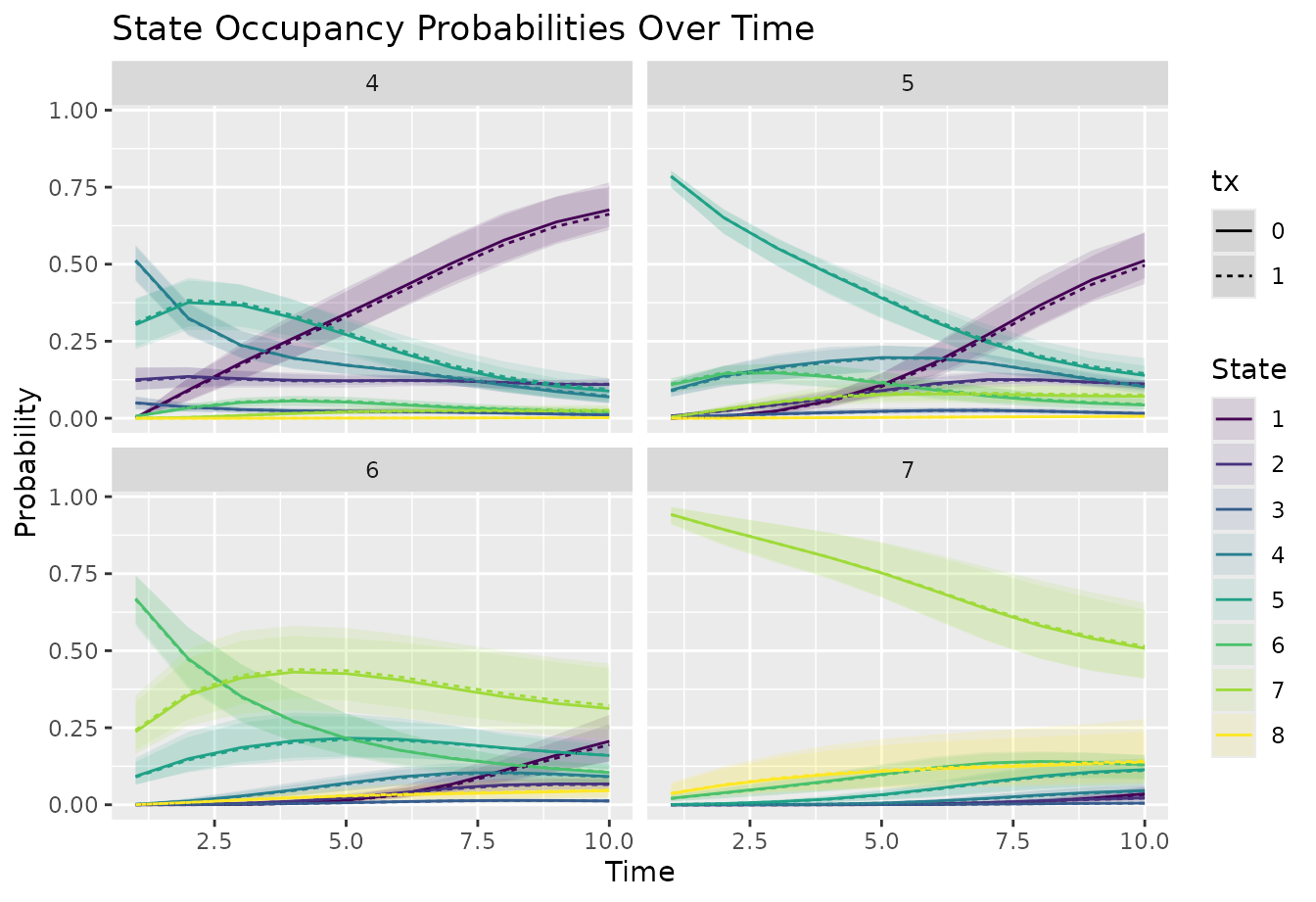
Each panel shows one starting state. Subgroups with few patients have wider intervals.

plot_sops(
  sop_fwb,
  facet_var = "starting_state",
  linetype_var = "tx"
)

Compare time benefit by subgroup

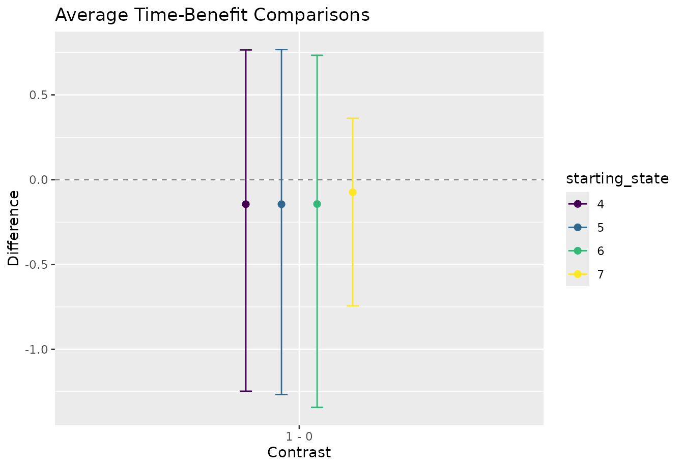
Time benefit summarizes the whole ordinal scale in one number: on each day, the probability that a patient would be in a better state under treatment than under control, minus the probability of a worse state, summed over days. See vignette("many-levels-previous-state-spline") for a fuller explanation. With by = "starting_state", it is reported separately for each starting state.

tb_fwb <- avg_comparisons(
  fit,
  times = seq_len(FOLLOW_UP),
  variables = list(tx = c(0, 1)),
  estimand = "time_benefit",
  absorb = ABSORB,
  by = "starting_state"
) |>
  inferences(
    method = "fwb",
    n_draws = N_BOOT,
    workers = 1,
    return_draws = TRUE
  )

plot_comparisons(tb_fwb, color_var = "starting_state")