Second-Order SOPs with orm_markov()
Source:vignettes/second-order-orm-sops.Rmd
second-order-orm-sops.RmdA first-order transition model predicts today’s state from yesterday’s state alone. Sometimes the state two days ago carries extra information: a patient who has just improved may be more likely to keep improving than one who has been stable. A second-order model captures this by including both previous states as predictors.
This article fits a second-order model with orm_markov()
and shows the one extra argument needed downstream: p2_var,
which names the column holding the state two days back. Every function
that computes model-based probabilities (avg_sops(),
avg_comparisons(), and the diagnostic plots) needs it, so
that it chains predictions through both previous states.
Data
We simulate 200 patients over 14 days with
sim_markov("actt2"), which uses the eight-state NIAID scale
described in vignette("full-po-sops"). The simulated data
contain the previous state, yprev, but not the state two
days back, so we construct that column, ypprev, by shifting
yprev by one day within each patient. The simulation
records only one state before day 1, so on day 1 we set
ypprev equal to yprev.
library(mostr)
library(ggplot2)
library(rms)

N_PATIENTS <- 200
FOLLOW_UP <- 14
SEED <- 20260529
STATE_LEVELS <- as.character(1:8)
ABSORB <- "8"

raw_data <- sim_markov(
  "actt2",
  n_patients = N_PATIENTS,
  follow_up_time = FOLLOW_UP,
  treatment_effect = log(0.8),
  seed = SEED
)

model_data <- prepare_markov_data(
  raw_data,
  absorbing_state = as.integer(ABSORB),
  factor_previous = TRUE
)
model_data <- model_data[order(model_data$id, model_data$time), ]

# State two days back: yprev shifted by one day, repeating the first value.
model_data$ypprev <- ave(
  model_data$yprev,
  model_data$id,
  FUN = function(x) c(x[1], head(x, -1))
)
model_data$ypprev <- factor(model_data$ypprev, levels = levels(model_data$yprev))

head(model_data[c("id", "time", "tx", "ypprev", "yprev", "y")])
#> id time tx ypprev yprev y
#> 1 1 1 0 5 5 5
#> 2 1 2 0 5 5 4
#> 3 1 3 0 5 4 4
#> 4 1 4 0 4 4 4
#> 5 1 5 0 4 4 2
#> 6 1 6 0 4 2 2Fit the model
The model includes both previous states as factors. It also lets the
effect of each previous state change linearly over time through the
%ia% interaction terms, rms’s operator for restricted
interactions.
dd <- datadist(model_data)
options(datadist = "dd")

fit_second <- orm_markov(
  y ~ tx + rcs(time, 4) + yprev + ypprev + time %ia% yprev + time %ia% ypprev,
  data = model_data,
  id_var = "id",
  opt_method = "LM",
  scale = TRUE,
  maxit = 100
)

fit_second
Show output
#> Logistic (Proportional Odds) Ordinal Regression Model
#>
#> rms::orm(formula = y ~ tx + rcs(time, 4) + yprev + ypprev + time %ia%
#>     yprev + time %ia% ypprev, data = model_data, opt_method = "LM",
#>     scale = TRUE, maxit = 100, x = TRUE, y = TRUE)
#>
#>
#> Frequencies of Responses
#>
#>   1   2   3   4   5   6   7   8
#> 801 224  27 275 735 308 368   9
#>
#>                          Model Likelihood               Discrimination    Rank Discrim.
#>                                Ratio Test                      Indexes          Indexes
#> Obs            2747    LR chi2    6050.11    R2                  0.919    rho     0.939
#> ESS          2611.6    d.f.            28    R2(28,2747)         0.888    Dxy     0.919
#> Distinct Y        8    Pr(> chi2) <0.0001    R2(28,2611.6)       0.900
#> Cluster on  cluster                          |Pr(Y>=median)-0.5| 0.422
#> Clusters        200
#> Median Y          5
#> max |deriv|   1e-05
#>
#>                 Coef     S.E.   Wald Z Pr(>|Z|)
#> y>=2              0.3527 0.8026   0.44 0.6603
#> y>=3             -4.3898 1.0626  -4.13 <0.0001
#> y>=4             -4.6864 1.0706  -4.38 <0.0001
#> y>=5             -6.8208 1.0748  -6.35 <0.0001
#> y>=6            -11.2681 1.0727 -10.50 <0.0001
#> y>=7            -15.1409 1.0965 -13.81 <0.0001
#> y>=8            -21.7012 1.1534 -18.81 <0.0001
#> tx               -0.1933 0.1029  -1.88 0.0604
#> time             -0.4322 0.0912  -4.74 <0.0001
#> time'             0.6857 0.1983   3.46 0.0005
#> time''           -1.3025 0.5294  -2.46 0.0139
#> yprev=2          -1.2562 1.5061  -0.83 0.4042
#> yprev=3           4.1293 2.0376   2.03 0.0427
#> yprev=4           5.1400 1.8554   2.77 0.0056
#> yprev=5           8.3461 1.9124   4.36 <0.0001
#> yprev=6          13.0841 1.9894   6.58 <0.0001
#> yprev=7          17.8829 2.1360   8.37 <0.0001
#> ypprev=2         -1.0141 1.1879  -0.85 0.3933
#> ypprev=3         -1.1976 1.9854  -0.60 0.5464
#> ypprev=4          1.4581 1.8616   0.78 0.4335
#> ypprev=5          1.2469 1.8837   0.66 0.5080
#> ypprev=6          1.0837 1.9714   0.55 0.5825
#> ypprev=7          1.1778 2.1683   0.54 0.5870
#> time * yprev=2    0.1011 0.1328   0.76 0.4465
#> time * yprev=3    0.1996 0.2216   0.90 0.3676
#> time * yprev=4    0.2528 0.1784   1.42 0.1566
#> time * yprev=5    0.2482 0.1904   1.30 0.1923
#> time * yprev=6    0.2248 0.2069   1.09 0.2772
#> time * yprev=7    0.3044 0.2237   1.36 0.1736
#> time * ypprev=2   0.0781 0.1123   0.70 0.4867
#> time * ypprev=3   0.1118 0.1991   0.56 0.5744
#> time * ypprev=4  -0.1699 0.1868  -0.91 0.3632
#> time * ypprev=5  -0.1750 0.1920  -0.91 0.3623
#> time * ypprev=6  -0.1899 0.2102  -0.90 0.3665
#> time * ypprev=7  -0.1684 0.2299  -0.73 0.4637
Estimate state occupancy probabilities
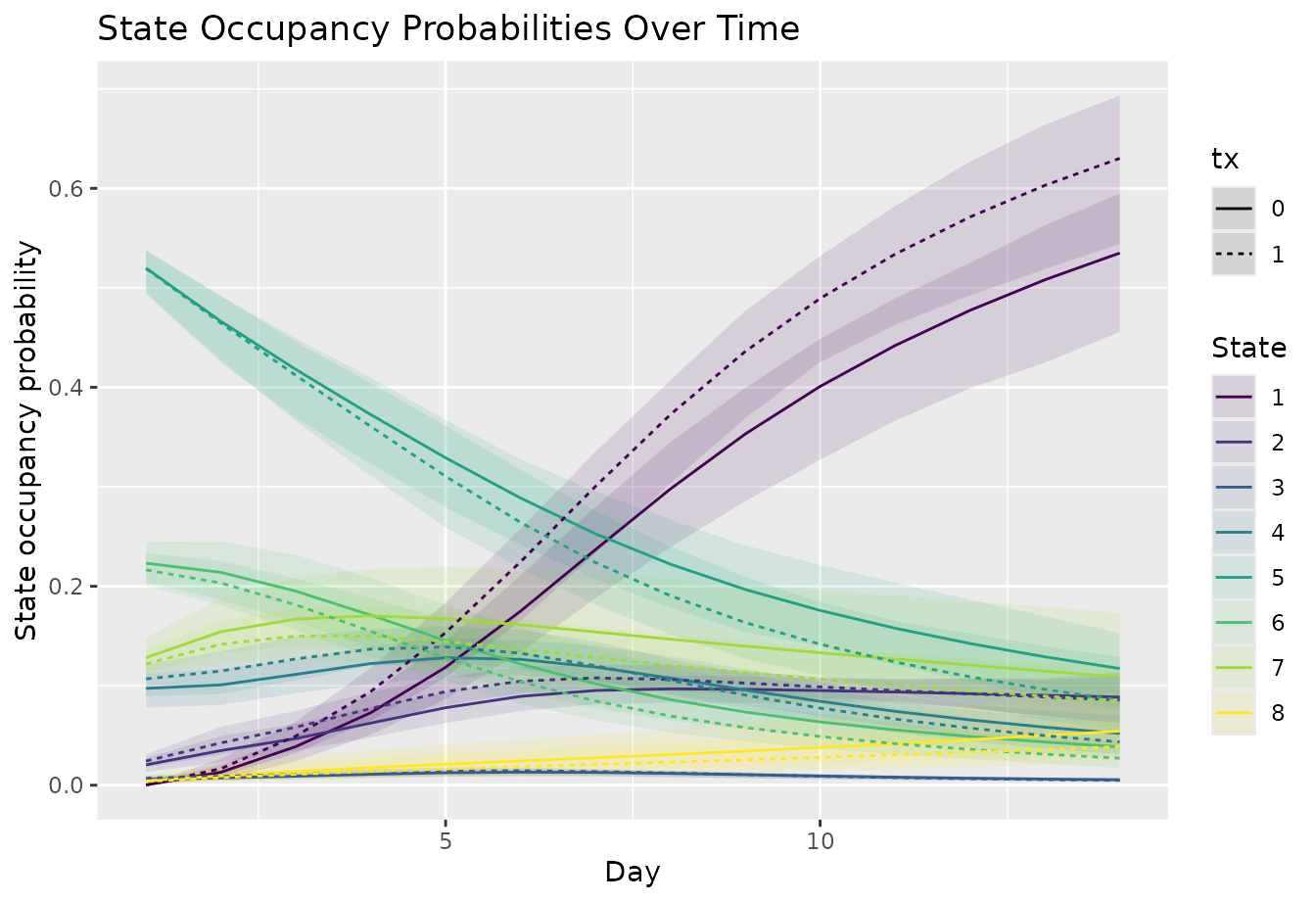
Passing p2_var = "ypprev" switches
avg_sops() from the first-order to the second-order
calculation described below. Analytical
confidence intervals are available only for first-order models, so we
use simulation from the coefficients’ multivariate normal distribution
(method = "mvn", the default). We use only 50 draws to keep
the example fast; use more, such as 1,000, in a real analysis.
sop_second <- avg_sops(
  fit_second,
  variables = list(tx = c(0, 1)),
  times = seq_len(FOLLOW_UP),
  y_levels = fit_second$yunique,
  absorb = ABSORB,
  p2_var = "ypprev"
) |>
  inferences(n_draws = 50)

head(sop_second)
#> time state tx estimate std.error conf.low conf.high
#> 1 1 1 0 0.0002023748 0.0001445127 4.875267e-05 0.000569765
#> 2 2 1 0 0.0130739206 0.0039853814 5.945094e-03 0.020963710
#> 3 3 1 0 0.0388085709 0.0074072188 2.403663e-02 0.050183309
#> 4 4 1 0 0.0728746386 0.0121160432 5.063010e-02 0.091988188
#> 5 5 1 0 0.1185248139 0.0177428109 8.662153e-02 0.145138114
#> 6 6 1 0 0.1749012033 0.0235350124 1.334699e-01 0.210853122
plot_sops(
  sop_second,
  geom = "line",
  facet_var = NULL,
  linetype_var = "tx"
) +
  labs(
    x = "Day",
    y = "State occupancy probability"
  )
Compare time in groups of states
state_sets groups states before comparing them. Here we
compare the expected number of days spent at home (states 1–2), in
hospital without high-flow oxygen or ventilation (3–5), on high-flow
oxygen or ventilation (6–7), and dead (8). Each estimate is treated
minus control.
tis_second <- avg_comparisons(
  fit_second,
  estimand = "time_in_state",
  state_sets = list(1:2, 3:5, 6:7, 8),
  variables = list(tx = c(0, 1)),
  times = seq_len(FOLLOW_UP),
  y_levels = fit_second$yunique,
  absorb = ABSORB,
  p2_var = "ypprev"
) |>
  inferences(n_draws = 100)

plot_comparisons(tis_second)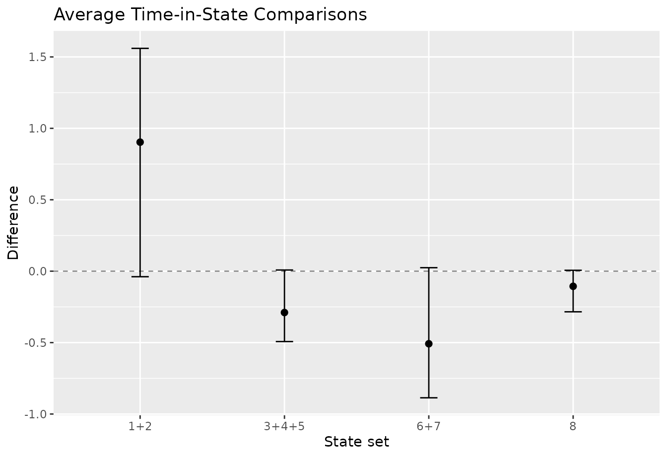
How the probabilities are calculated
This section extends the calculation in
vignette("full-po-sops") to two previous states. You can
skip it on a first reading.
Let \(i = 1,\ldots,n\) index patients, \(t = 1,\ldots,d\) index follow-up days, and \(Y_{it}\) be patient \(i\)’s state on day \(t\), one of \(K\) ordered states. The vector \(\mathbf{x}_{it}\) holds treatment, time, and other covariates on day \(t\), and \(\mathbf{x}_{i,1:t}\) holds their values up to day \(t\). Two starting states are needed, \(Y_{i,-1}\) and \(Y_{i0}\); as noted above, this example sets \(Y_{i,-1} = Y_{i0}\). The state occupancy probability (SOP) for state \(l\) is
\[ S_{it}(l) = \Pr(Y_{it} = l \mid \mathbf{x}_{i,1:t}, Y_{i,-1}, Y_{i0}). \]
The fitted model supplies the probability of moving to state \(l\) given the states \(h\) two days back and \(k\) one day back,
\[ T_{it}(l \mid h, k) = \Pr(Y_{it} = l \mid Y_{i,t-2} = h, Y_{i,t-1} = k, \mathbf{x}_{it}), \]
obtained by setting ypprev to \(h\), yprev to \(k\), and time to \(t\). If \(k\) is an absorbing state, the model is not
used: \(T_{it}(l \mid h, k)\) is 1 for
\(l = k\) and 0 otherwise, whatever
\(h\) is.
Because tomorrow depends on the last two states, the SOPs alone are not enough to take the next step. Instead, the calculation tracks the joint probability of the last two states,
\[ J_{it}(k,l) = \Pr(Y_{i,t-1} = k, Y_{it} = l \mid \mathbf{x}_{i,1:t}, Y_{i,-1}, Y_{i0}). \]
On the first day, only the observed starting states are possible:
\[ J_{i1}(k,l) = \mathbb{1}\{k = Y_{i0}\}\, T_{i1}(l \mid Y_{i,-1}, Y_{i0}), \]
where \(\mathbb{1}\{\cdot\}\) is 1 when its condition holds and 0 otherwise. On each later day, the new joint probability adds up the paths through every possible state \(h\) two days back:
\[ J_{it}(k,l) = \sum_{h=1}^{K} J_{i,t-1}(h,k)\, T_{it}(l \mid h,k), \qquad t = 2,\ldots,d. \]
The SOP is the probability of the current state regardless of the previous one:
\[ S_{it}(l) = \sum_{k=1}^{K} J_{it}(k,l). \]
As in the first-order case, mostr performs these updates for all patients at once, carries forward probability in absorbing states without predicting from them, and averages the patient-level SOPs within each treatment arm. It computes the probabilities exactly rather than by simulating individual trajectories.
Check the model against the data
The diagnostics compare observed summaries with those implied by the
model, as explained in vignette("full-po-sops"). The
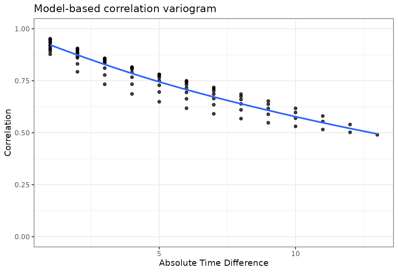
model-based plots also need p2_var = "ypprev". Because a
second-order model remembers more of each patient’s history, it can
reproduce correlations that persist over longer gaps than a first-order
model allows; the variogram is the most direct place to see this. The
transition heatmaps use at most sixteen evenly spaced days.
diagnostic_times <- unique(round(seq(1, FOLLOW_UP, length.out = min(16L, FOLLOW_UP))))

plot_transitions(
  raw_data,
  times = diagnostic_times,
  y_levels = STATE_LEVELS,
  show_values = FALSE
) +
  labs(title = "Observed transition proportions")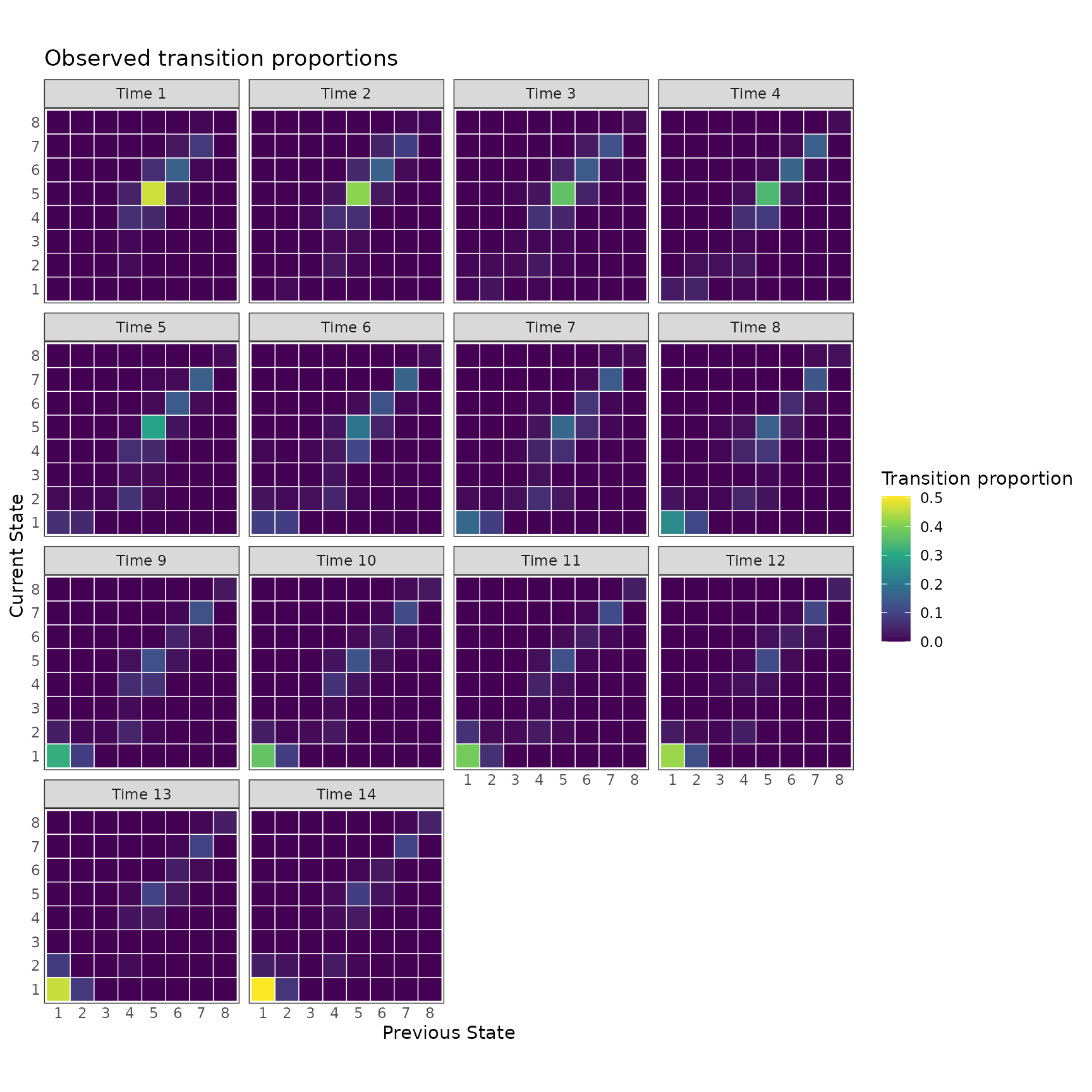
plot_transitions(
  fit_second,
  times = diagnostic_times,
  y_levels = fit_second$yunique,
  absorb = ABSORB,
  p2_var = "ypprev",
  show_values = FALSE
) +
  labs(title = "Model-based transition proportions")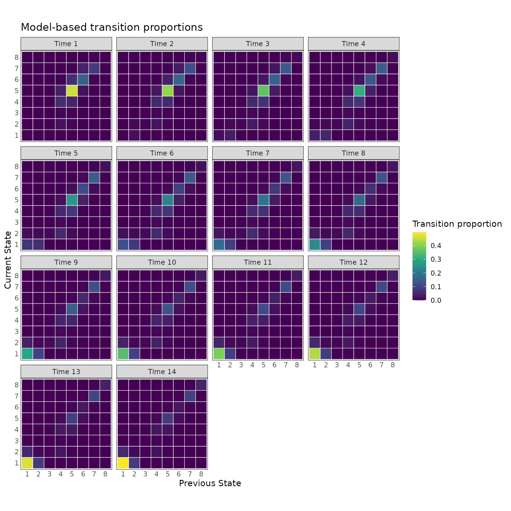
plot_correlation(
  fill_limits = c(0, 1),
  raw_data,
  times = seq_len(FOLLOW_UP),
  show_values = FALSE
) +
  labs(title = "Observed state correlations")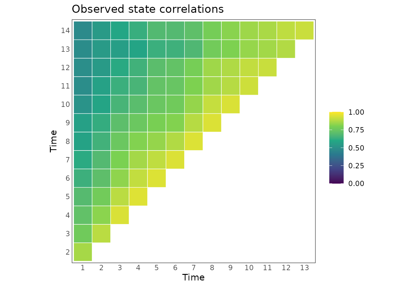
plot_correlation(
  fill_limits = c(0, 1),
  fit_second,
  times = seq_len(FOLLOW_UP),
  y_levels = fit_second$yunique,
  absorb = ABSORB,
  p2_var = "ypprev",
  show_values = FALSE
) +
  labs(title = "Model-based state correlations")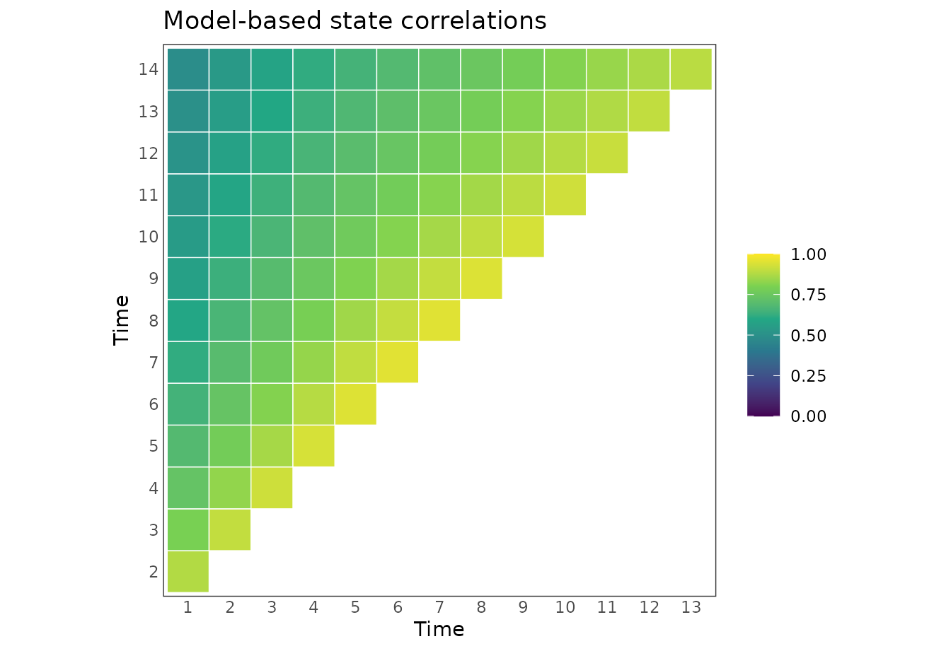
plot_variogram(
  raw_data,
  times = seq_len(FOLLOW_UP)
) +
  labs(title = "Observed correlation variogram")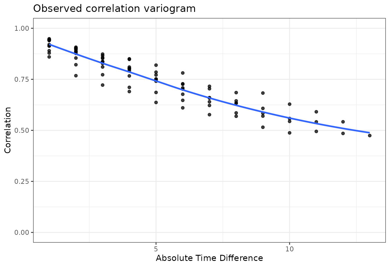
plot_variogram(
  fit_second,
  times = seq_len(FOLLOW_UP),
  y_levels = fit_second$yunique,
  absorb = ABSORB,
  p2_var = "ypprev"
) +
  labs(title = "Model-based correlation variogram")