Partial Proportional-Odds SOPs with vglm

A proportional-odds model assumes that each covariate shifts the odds of being in a worse state by the same factor at every cut-point of the ordinal scale. For example, the effect of time on the odds of being in hospital or worse is assumed to equal its effect on the odds of death. When this assumption is doubtful for some covariates, a partial proportional-odds model lets their effects differ between cut-points while keeping proportional odds for the others.

This article fits both kinds of model to the same data with vglm_markov(): a full proportional-odds model, and a partial proportional-odds model in which the effect of time differs between the cut-points. We compare how well the two models fit, and how closely each reproduces the observed state occupancy probabilities (SOPs), transitions, and correlations between days.

Simulate data

We simulate 1,000 patients over 28 days with sim_markov("violet"). Its trajectories resemble those of the VIOLET trial of vitamin D3 in critically ill adults, and each patient’s starting state, age, and SOFA (Sequential Organ Failure Assessment) score are drawn from the VIOLET patients. There are four states:

State	Meaning
1	At home
2	In hospital or another health care facility
3	On a ventilator or with acute respiratory distress syndrome (ARDS)
4	Dead

Death is absorbing. Treated patients (tx = 1) have 0.8 times the odds of being in a worse state on any day.

The simulator itself is a partial proportional-odds model, described in ?violet_preset. Time enters as a straight line whose slope changes after day 2, and both slopes differ between the three cut-points. During the first two days, each day lowers the log odds of being in hospital or worse by 1.315, so many patients go home, but raises the log odds of death by 0.412. After day 2 all three slopes are close to zero. A single time effect shared by all cut-points cannot describe both trends, so we can check which model recovers this structure.

library(mostr)
library(ggplot2)
library(patchwork)
library(rms)
library(VGAM)

N_PATIENTS <- 1000
FOLLOW_UP <- 28
SEED <- 20261009
STATE_LEVELS <- as.character(1:4)
ABSORB <- "4"

raw_data <- sim_markov(
  "violet",
  n_patients = N_PATIENTS,
  follow_up_time = FOLLOW_UP,
  treatment_effect = log(0.8),
  seed = SEED
)

model_data <- prepare_markov_data(raw_data, absorbing_state = 4)

Fit the proportional-odds model

Both models use treatment, the previous state, age, SOFA score, and the same time trend as the simulator: time and pmax(time - 2, 0), the number of days after day 2. Together they form a straight line whose slope changes after day 2.

In VGAM, cumulative(reverse = TRUE) models the odds of worse (higher) states, and parallel = TRUE requests proportional odds for every term.

form <- ordered(y) ~ tx + time + pmax(time - 2, 0) + yprev + age + sofa

fit_po <- vglm_markov(
  form,
  family = VGAM::cumulative(reverse = TRUE, parallel = TRUE),
  data = model_data,
  id_var = "id"
)

Specify which effects may vary

VGAM expresses partial proportional odds through constraint matrices. The model has one linear predictor per cut-point; with four states there are three, for “state 2 or worse”, “state 3 or worse”, and “state 4” (dead). Each model term has a constraint matrix with one row per cut-point and one column per coefficient for that term:

a single column of ones gives one coefficient shared by all cut-points, which is proportional odds;
an identity matrix, with one column per cut-point, gives the term a separate coefficient at every cut-point.

The easiest way to obtain a valid set of constraint matrices is to fit the proportional-odds model first and edit its constraints. We change two things:

The two time terms get identity matrices, so that each cut-point has its own time slopes, as in the simulator.
The fitted model lists a separate constraint for each dummy variable of the factor yprev. The constraints we supply must instead be named by the formula term, so we replace these entries with a single yprev entry with proportional odds.

constraints <- fit_po$vglm_fit@constraints

# One row per cut-point: three for four states.
n_thresholds <- nrow(constraints[["time"]])

# Replace the per-dummy yprev constraints with one term-level entry.
yprev_terms <- grep("^yprev", names(constraints), value = TRUE)
constraints[yprev_terms] <- NULL
constraints[["yprev"]] <- cbind(PO_effect = rep(1, n_thresholds))

# A separate time slope at each cut-point.
time_terms <- c("time", "pmax(time - 2, 0)")
constraints[time_terms] <- list(diag(n_thresholds))
constraints[["time"]]

#>      [,1] [,2] [,3]
#> [1,]    1    0    0
#> [2,]    0    1    0
#> [3,]    0    0    1

Fit the partial proportional-odds model

We refit the model with these constraints. parallel = FALSE tells VGAM not to impose proportional odds on every term, so that our constraint matrices decide instead. Starting from the proportional-odds fit’s linear predictors (etastart) helps the fit converge. The final line stores the constraint list itself, rather than the name constraints, in the model call, so that code that later re-evaluates the call does not depend on this variable.

fit_ppo <- vglm_markov(
  form,
  family = VGAM::cumulative(reverse = TRUE, parallel = FALSE),
  data = model_data,
  id_var = "id",
  constraints = constraints,
  etastart = fit_po$vglm_fit@predictors
)
fit_ppo$vglm_fit@call$constraints <- constraints

VGAM numbers the coefficients of a term by the columns of its constraint matrix, so the time slopes of the partial proportional-odds model end in :1 for “state 2 or worse”, :2 for “state 3 or worse”, and :3 for death. The proportional-odds model has one slope for each time term. We compare both with the slopes used by the simulator:

coef_po <- coef(fit_po$vglm_fit)
coef_ppo <- coef(fit_ppo$vglm_fit)

data.frame(
  term = rep(time_terms, each = n_thresholds),
  cutoff = rep(c("hospital or worse", "ventilator/ARDS or dead", "dead"), 2),
  PO = rep(coef_po[time_terms], each = n_thresholds),
  PPO = coef_ppo[paste0(rep(time_terms, each = n_thresholds), ":", 1:3)],
  simulated = c(-1.315, -0.481, 0.412, 1.384, 0.525, -0.410),
  row.names = NULL
)

#>                term                  cutoff         PO        PPO simulated
#> 1              time       hospital or worse -0.7992013 -1.4110546    -1.315
#> 2              time ventilator/ARDS or dead -0.7992013 -0.5612482    -0.481
#> 3              time                    dead -0.7992013  0.3639808     0.412
#> 4 pmax(time - 2, 0)       hospital or worse  0.8537469  1.4796290     1.384
#> 5 pmax(time - 2, 0) ventilator/ARDS or dead  0.8537469  0.6106199     0.525
#> 6 pmax(time - 2, 0)                    dead  0.8537469 -0.3588023    -0.410

The partial proportional-odds slopes are close to the simulated ones, while the proportional-odds model replaces them with one compromise slope for each time term. Both models estimate the treatment effect well; the simulated value is \(\log(0.8) \approx -0.22\):

c(PO = coef_po[["tx"]], PPO = coef_ppo[["tx"]], simulated = log(0.8))

#>         PO        PPO  simulated 
#> -0.2041328 -0.2037432 -0.2231436

Compare model fit

The Akaike information criterion, AIC(), measures how well a model fits the data while penalizing each extra coefficient by 2 units; lower values are better. The Bayesian information criterion, BIC(), penalizes each coefficient by the logarithm of the number of observations instead. A difference of more than about 10 is usually regarded as strong evidence for the model with the lower value. Because the proportional-odds model is the partial proportional-odds model with the time slopes forced to be equal, we can also compare them with a likelihood ratio test, VGAM::lrtest().

data.frame(
  model = c("Proportional odds", "Partial proportional odds"),
  coefficients = c(length(coef_po), length(coef_ppo)),
  AIC = c(AIC(fit_po$vglm_fit), AIC(fit_ppo$vglm_fit)),
  BIC = c(BIC(fit_po$vglm_fit), BIC(fit_ppo$vglm_fit))
)

#>                       model coefficients      AIC      BIC
#> 1         Proportional odds           10 9181.762 9263.240
#> 2 Partial proportional odds           14 9152.277 9266.347

VGAM::lrtest(fit_ppo$vglm_fit, fit_po$vglm_fit)

#> Likelihood ratio test
#> 
#> Model 1: ordered(y) ~ tx + time + pmax(time - 2, 0) + yprev + age + sofa
#> Model 2: ordered(y) ~ tx + time + pmax(time - 2, 0) + yprev + age + sofa
#>     #Df  LogLik Df  Chisq Pr(>Chisq)    
#> 1 76597 -4562.1                         
#> 2 76601 -4580.9  4 37.485  1.431e-07 ***
#> ---
#> Signif. codes:  0 '***' 0.001 '**' 0.01 '*' 0.05 '.' 0.1 ' ' 1

AIC and the likelihood ratio test strongly favour the partial proportional-odds model. BIC is about the same for both models: with about 25,500 daily observations it charges about 10 units for each of the four extra coefficients, which nearly cancels their improvement in fit.

Compare state occupancy probabilities

avg_sops() estimates, for each arm, the probability of each state on each day, averaged over the patients’ observed starting states and covariates (see vignette("full-po-sops")). We compare both models’ estimates with the observed proportion of patients in each state, separately for each arm. Only point estimates are needed here, so we do not call inferences().

sop_args <- list(
  variables = list(tx = c(0, 1)),
  times = seq_len(FOLLOW_UP),
  y_levels = STATE_LEVELS,
  absorb = ABSORB
)
sop_po <- do.call(avg_sops, c(list(fit_po), sop_args))
sop_ppo <- do.call(avg_sops, c(list(fit_ppo), sop_args))

observed <- as.data.frame(
  prop.table(
    table(
      tx = raw_data$tx,
      time = raw_data$time,
      state = factor(raw_data$y, levels = STATE_LEVELS)
    ),
    margin = c(1, 2)
  ),
  responseName = "estimate"
)

sop_comparison <- rbind(
  data.frame(source = "Observed", observed[, c("tx", "time", "state", "estimate")]),
  data.frame(source = "Proportional odds", as.data.frame(sop_po)[, c("tx", "time", "state", "estimate")]),
  data.frame(source = "Partial proportional odds", as.data.frame(sop_ppo)[, c("tx", "time", "state", "estimate")])
)
sop_comparison$time <- as.integer(as.character(sop_comparison$time))
sop_comparison$source <- factor(
  sop_comparison$source,
  levels = c("Observed", "Proportional odds", "Partial proportional odds")
)

ggplot(
  subset(sop_comparison, tx == 0),
  aes(time, estimate, colour = source, linetype = source)
) +
  geom_line() +
  facet_wrap(~state, scales = "free_y", labeller = label_both, ncol = 2) +
  labs(
    x = "Day",
    y = "State occupancy probability",
    colour = NULL,
    linetype = NULL,
    title = "Control arm"
  ) +
  theme(legend.position = "bottom")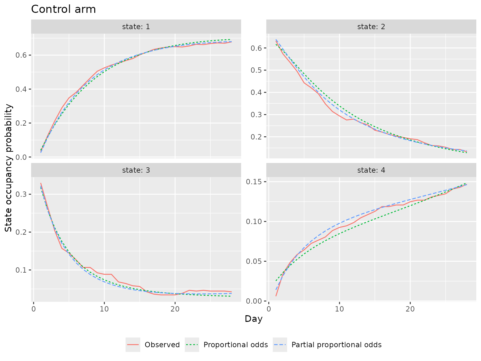

Both models follow the observed proportions closely, but the proportional-odds model makes two systematic errors. It sends patients home too slowly in the second week, leaving about 3 percentage points too many in hospital, and it puts too many deaths on day 1 and too few during the second and third weeks. The mean absolute difference from the observed proportions over all days, states, and arms summarizes this:

sop_wide <- reshape(
  sop_comparison,
  idvar = c("tx", "time", "state"),
  timevar = "source",
  direction = "wide"
)
c(
  `Proportional odds` = mean(abs(
    sop_wide$`estimate.Proportional odds` - sop_wide$estimate.Observed
  )),
  `Partial proportional odds` = mean(abs(
    sop_wide$`estimate.Partial proportional odds` - sop_wide$estimate.Observed
  ))
)

#>         Proportional odds Partial proportional odds 
#>               0.011644728               0.007905667

Compare transitions

plot_transitions() shows, for selected days, the proportion of all patients who move from each previous state (x-axis) to each current state (y-axis). For the observed data these are counts divided by the number of patients; for a model they are the expected proportions implied by its transition probabilities.

transition_sources <- list(
  Observed = plot_transitions(
    raw_data,
    times = seq_len(FOLLOW_UP),
    y_levels = STATE_LEVELS
  ),
  `Proportional odds` = plot_transitions(
    fit_po,
    times = seq_len(FOLLOW_UP),
    y_levels = STATE_LEVELS,
    absorb = ABSORB
  ),
  `Partial proportional odds` = plot_transitions(
    fit_ppo,
    times = seq_len(FOLLOW_UP),
    y_levels = STATE_LEVELS,
    absorb = ABSORB
  )
)
transitions <- do.call(rbind, Map(
  function(plot, source) {
    data.frame(
      source = source,
      time = as.integer(as.character(plot$data$.time_key)),
      previous_state = plot$data$previous_state,
      state = plot$data$state,
      estimate = plot$data$estimate
    )
  },
  transition_sources,
  names(transition_sources)
))
transitions$source <- factor(transitions$source, levels = names(transition_sources))

ggplot(
  subset(transitions, time %in% c(2, 7, 14, 28)),
  aes(previous_state, state, fill = estimate)
) +
  geom_tile(colour = "white") +
  facet_grid(source ~ time, labeller = labeller(time = function(x) paste("Day", x))) +
  scale_fill_viridis_c(trans = "sqrt", limits = c(0, NA)) +
  coord_equal() +
  labs(x = "Previous state", y = "Current state", fill = "Proportion")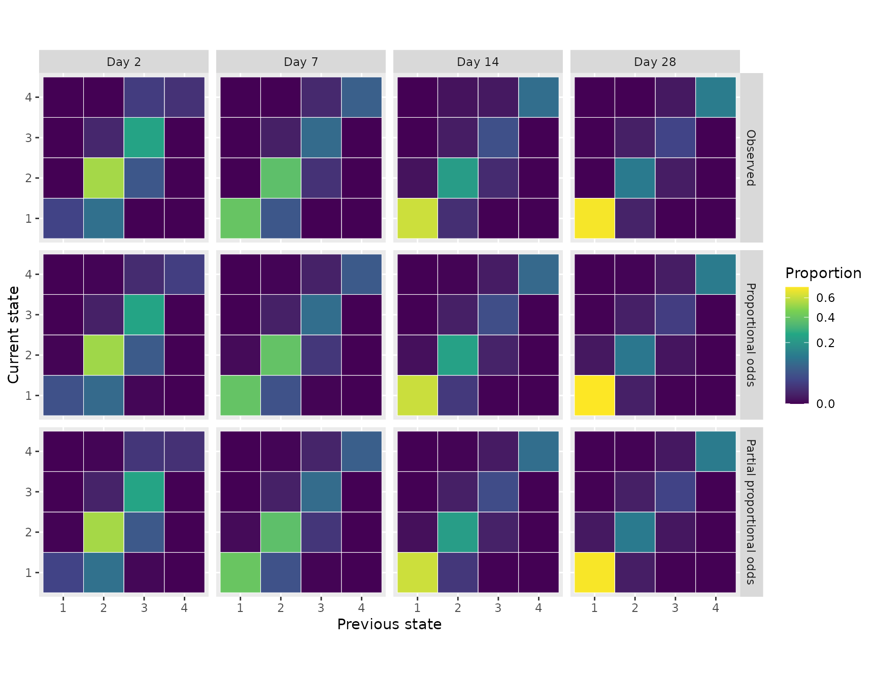

Most patients stay in their previous state, so the diagonal dominates all three rows. Differences between the models appear in the smaller off-diagonal proportions. The plotted values are easier to compare directly over time. For example, the proportion of patients who die on each day after being on a ventilator or with ARDS the day before:

ggplot(
  subset(transitions, previous_state == "3" & state == "4"),
  aes(time, estimate, colour = source, linetype = source)
) +
  geom_line() +
  labs(
    x = "Day",
    y = "Proportion of patients",
    colour = NULL,
    linetype = NULL,
    title = "Moves from ventilator or ARDS (state 3) to death (state 4)"
  )

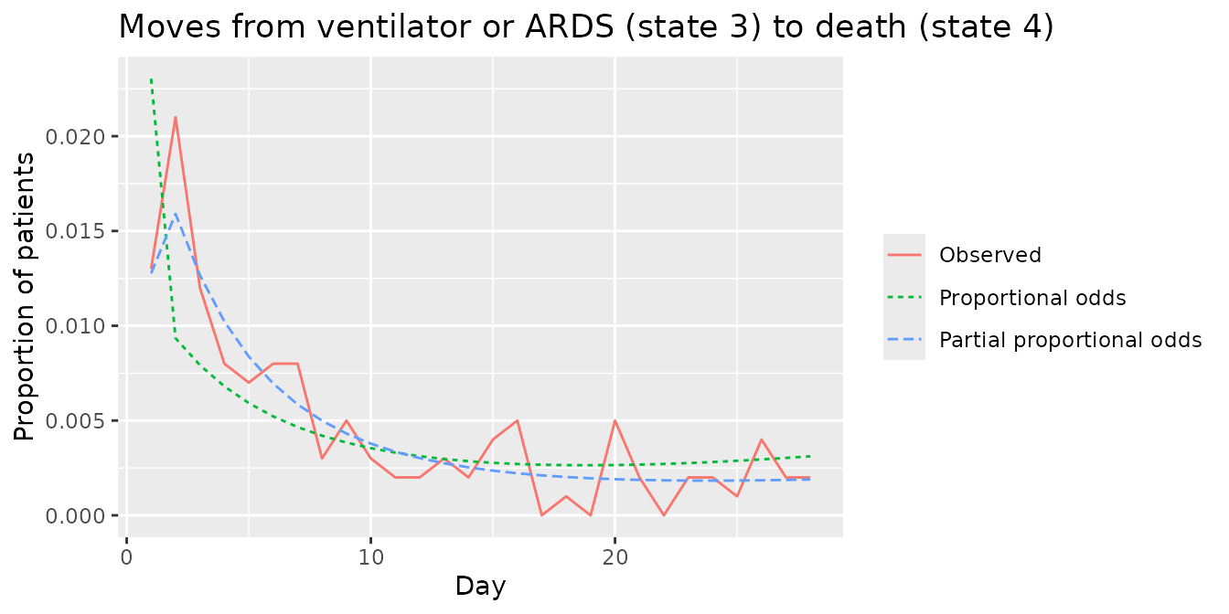
The proportional-odds model, which must give death the same time trend as leaving hospital, overestimates these deaths on day 1 and underestimates them during the following week. The partial proportional-odds model follows the observed proportions.

Compare correlations between days

plot_correlation() shows the Spearman rank correlation between patients’ states on every pair of days, from the observed data or implied by a model.

correlation_days <- seq(1, FOLLOW_UP, by = 3)

correlation_plots <- list(
  plot_correlation(
    raw_data,
    times = correlation_days,
    fill_limits = c(0, 1),
    show_values = FALSE
  ) +
    labs(title = "Observed"),
  plot_correlation(
    fit_po,
    times = correlation_days,
    y_levels = STATE_LEVELS,
    absorb = ABSORB,
    fill_limits = c(0, 1),
    show_values = FALSE
  ) +
    labs(title = "Proportional odds"),
  plot_correlation(
    fit_ppo,
    times = correlation_days,
    y_levels = STATE_LEVELS,
    absorb = ABSORB,
    fill_limits = c(0, 1),
    show_values = FALSE
  ) +
    labs(title = "Partial proportional odds")
)
wrap_plots(correlation_plots, nrow = 1) + plot_layout(guides = "collect")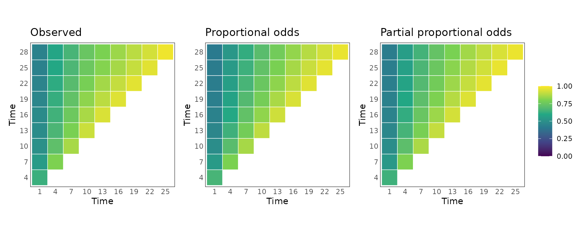

All three plots look almost the same. Correlations between days depend mainly on how strongly patients tend to stay in their previous state, which both models capture.

Compare treatment effects on time in each state

avg_comparisons() with estimand = "time_in_state" sums each arm’s daily SOPs over follow-up. The result is the expected number of days spent in each state, and the comparison reports treated minus control. A positive difference for state 1 means that treated patients are expected to spend more of the 28 days at home.

Analytical confidence intervals (method = "delta") are available only for full proportional-odds models, so for the partial proportional-odds model we use method = "mvn". It draws coefficient vectors from a multivariate normal distribution centered on the estimates, with the model’s covariance matrix, recomputes the result for each draw, and takes percentiles. We use only 100 draws to keep this example fast; use more, such as 1,000, in a real analysis.

tis_args <- list(
  estimand = "time_in_state",
  variables = list(tx = c(0, 1)),
  times = seq_len(FOLLOW_UP),
  y_levels = STATE_LEVELS,
  absorb = ABSORB
)

tis_po <- do.call(avg_comparisons, c(list(fit_po), tis_args)) |>
  inferences(method = "delta", vcov = "conditional")
tis_ppo <- do.call(avg_comparisons, c(list(fit_ppo), tis_args)) |>
  inferences(method = "mvn", n_draws = 100, seed = SEED)

tis_comparison <- rbind(
  data.frame(model = "Proportional odds", as.data.frame(tis_po)),
  data.frame(model = "Partial proportional odds", as.data.frame(tis_ppo))
)
tis_comparison$model <- factor(
  tis_comparison$model,
  levels = c("Proportional odds", "Partial proportional odds")
)
tis_comparison[, c("model", "state_set", "estimate", "conf.low", "conf.high")]

#>                       model state_set   estimate   conf.low  conf.high
#> 1         Proportional odds         1  1.8752285  0.8131048  2.9373522
#> 2         Proportional odds         2 -0.8244368 -1.2930746 -0.3557990
#> 3         Proportional odds         3 -0.3558708 -0.5712673 -0.1404743
#> 4         Proportional odds         4 -0.6949209 -1.0926051 -0.2972368
#> 5 Partial proportional odds         1  1.8786564  0.9946950  2.6749667
#> 6 Partial proportional odds         2 -0.8019359 -1.1346815 -0.4252286
#> 7 Partial proportional odds         3 -0.3483158 -0.5055796 -0.1772689
#> 8 Partial proportional odds         4 -0.7284046 -1.0733325 -0.3814286

ggplot(
  tis_comparison,
  aes(state_set, estimate, ymin = conf.low, ymax = conf.high, colour = model)
) +
  geom_hline(yintercept = 0, colour = "grey60") +
  geom_pointrange(position = position_dodge(width = 0.5)) +
  labs(
    x = "State",
    y = "Difference in days (treated - control)",
    colour = NULL
  ) +
  theme(legend.position = "bottom")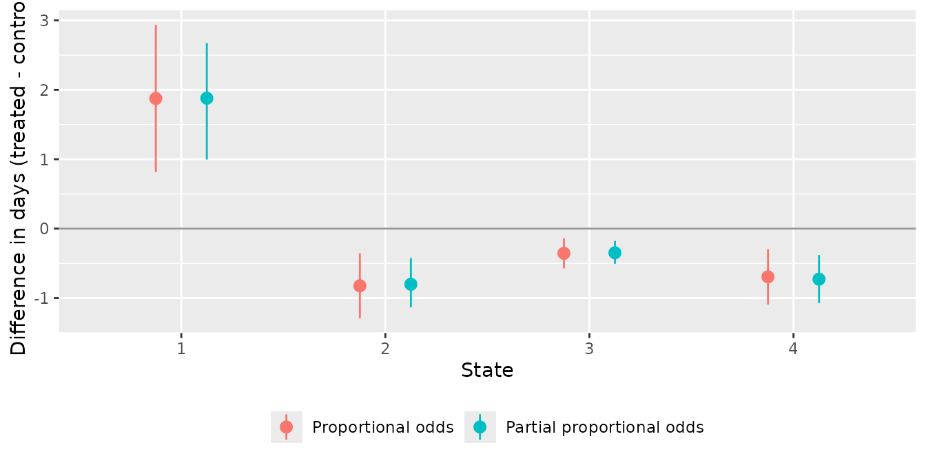

The two models give similar treatment effects even though their SOPs differ.

Partial Proportional-Odds SOPs with vglm_markov()